R Spatial
2026-03-25
Construire des flux reproductibles

Données spatiales
| Type d’objet | Description |
sf
|
stars
|
terra
|
|---|---|---|---|---|
| Vecteur | Où sont les entités? | |||
 Points Points
|
Emplacements discrets avec coordonnées et attributs. | ✓ | ✓ | |
 Lignes Lignes
|
Entités linéaires comme les routes, rivières ou tracés. | ✓ | ✓ | |
 Polygones Polygones
|
Surfaces comme les lacs, zones d’étude ou limites administratives. | ✓ | ✓ | |
| Raster | Quelle est la valeur à travers l’espace? | |||
 Rasters Rasters
|
Surfaces quadrillées avec des valeurs stockées dans des cellules. | ✓ | ✓ |
Une note sur les exercices
Choisissez votre parcours

Faites les deux niveaux!
Les participants plus avancés peuvent compléter les deux parcours, car il y aura des flux de travail avancés disponibles avec les points et les lignes.
Lire des données vectorielles
Simple feature collection with 1 feature and 1 field
Geometry type: POLYGON
Dimension: XY
Bounding box: xmin: -73 ymin: 46.55 xmax: -72.6 ymax: 47
Geodetic CRS: WGS 84
name geom
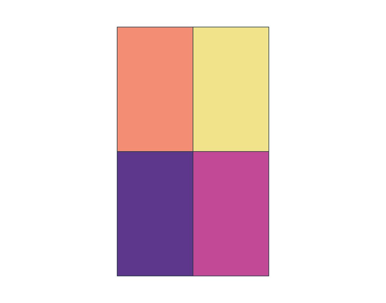
1 study_area POLYGON ((-73 46.55, -72.6 ...Simple feature collection with 4 features and 2 fields
Geometry type: POLYGON
Dimension: XY
Bounding box: xmin: -73 ymin: 46.55 xmax: -72.6 ymax: 47
Geodetic CRS: WGS 84
zone_id zone_type geom
1 NW forest POLYGON ((-73 46.775, -72.8...
2 NE urban POLYGON ((-72.8 46.775, -72...
3 SW wetland POLYGON ((-73 46.55, -72.8 ...
4 SE agriculture POLYGON ((-72.8 46.55, -72....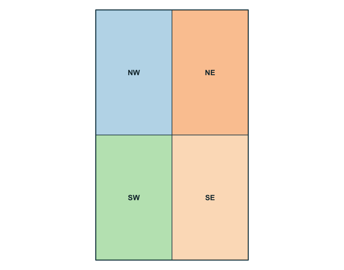

Convertir un tableau en points
Simple feature collection with 6 features and 8 fields
Geometry type: POINT
Dimension:     XY
Bounding box:  xmin: -72.92 ymin: 46.7 xmax: -72.72 ymax: 46.94
Geodetic CRS:  WGS 84
  obs_id track_id seq           timestamp    lon   lat    category value
1  OBS01        A   1 2026-03-01 08:00:00 -72.92 46.78       urban    14
2  OBS02        A   2 2026-03-01 09:00:00 -72.86 46.83       urban    16
3  OBS03        A   3 2026-03-01 10:00:00 -72.79 46.88      forest    21
4  OBS04        A   4 2026-03-01 11:00:00 -72.72 46.94      forest    24
5  OBS05        B   1 2026-03-02 08:00:00 -72.88 46.70 agriculture    11
6  OBS06        B   2 2026-03-02 09:00:00 -72.83 46.76 agriculture    13
              geometry
1 POINT (-72.92 46.78)
2 POINT (-72.86 46.83)
3 POINT (-72.79 46.88)
4 POINT (-72.72 46.94)
5  POINT (-72.88 46.7)
6 POINT (-72.83 46.76)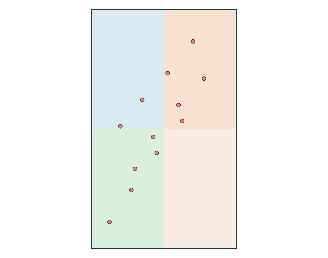
  obs_id track_id seq           timestamp    category value
1  OBS01        A   1 2026-03-01 08:00:00       urban    14
2  OBS02        A   2 2026-03-01 09:00:00       urban    16
3  OBS03        A   3 2026-03-01 10:00:00      forest    21
4  OBS04        A   4 2026-03-01 11:00:00      forest    24
5  OBS05        B   1 2026-03-02 08:00:00 agriculture    11
6  OBS06        B   2 2026-03-02 09:00:00 agriculture    13
Transformer le CRS
[1] "EPSG:32198" xmin ymin xmax ymax
-340347.4 299996.5 -318731.5 336605.7 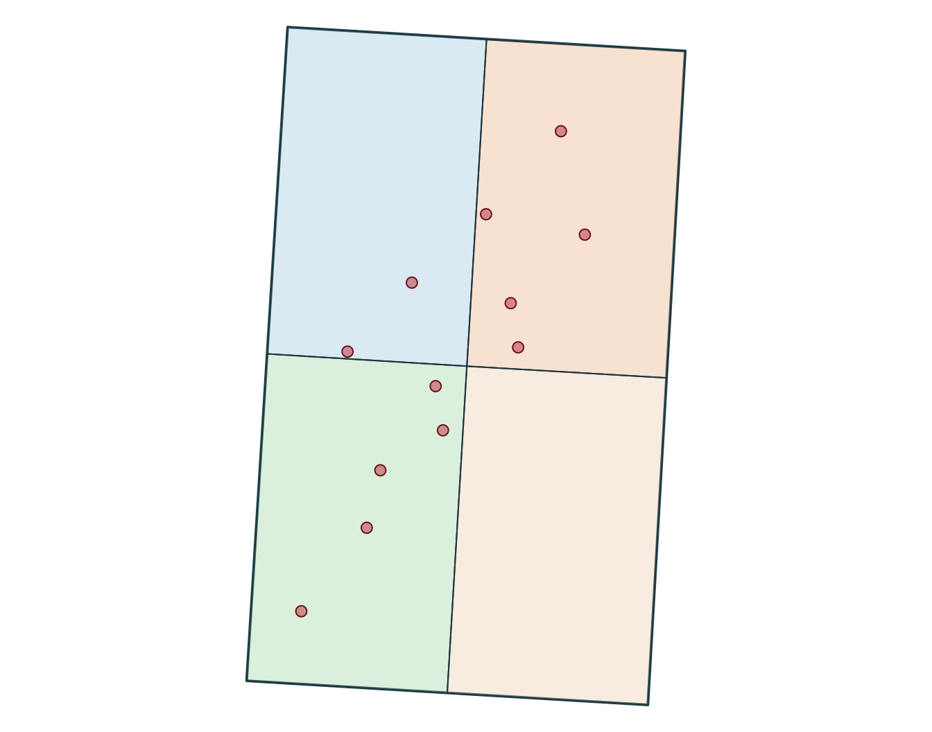
[1] "+proj=lcc +lat_0=44 +lon_0=-68.5 +lat_1=60 +lat_2=46 +x_0=0 +y_0=0 +datum=NAD83 +units=m +no_defs"SpatExtent : -340347.355525386, -318731.482880504, 299996.469057655, 336605.697992394 (xmin, xmax, ymin, ymax)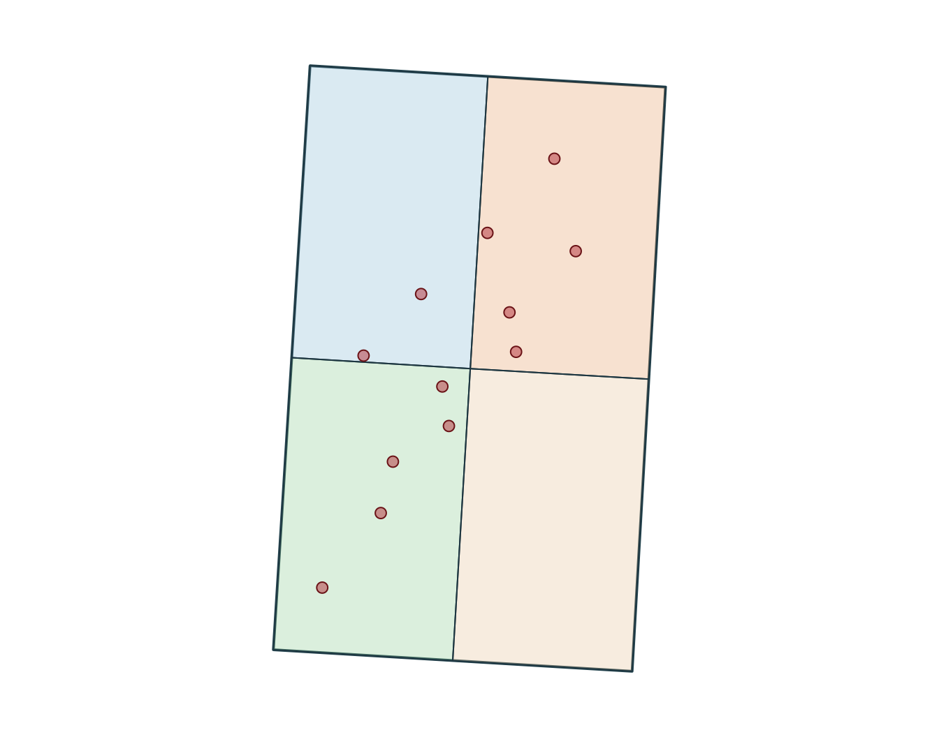
Mesures
Utilisez un CRS adapté lorsque vous avez besoin de distances, longueurs ou surfaces interprétables.
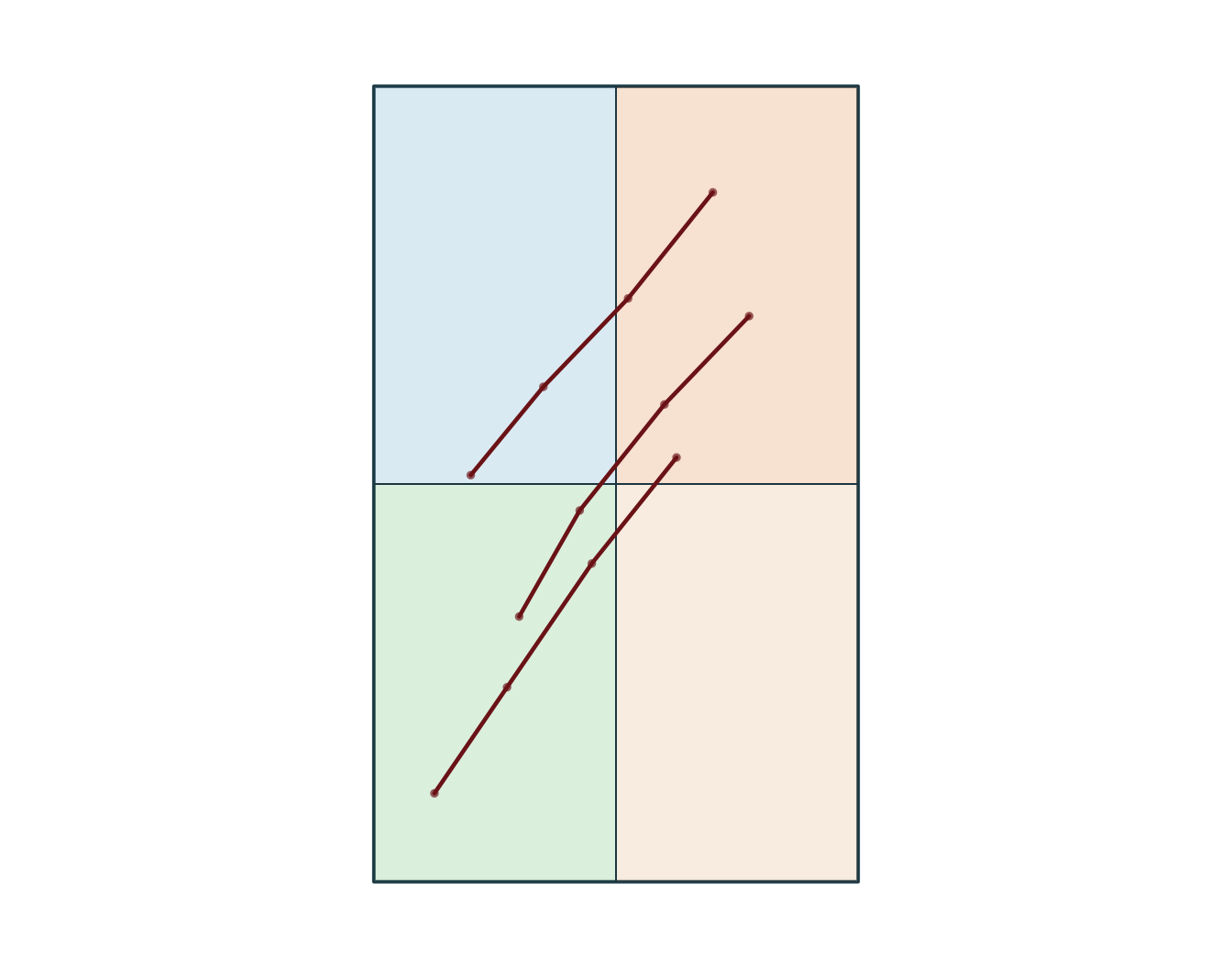
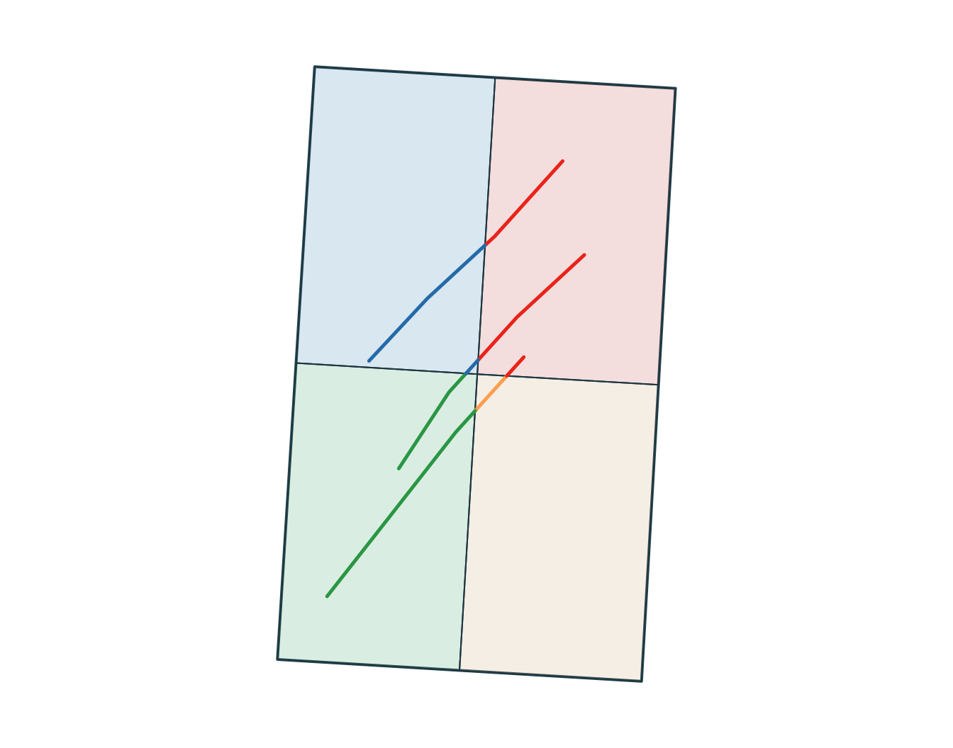
Convertir des points en lignes
Simple feature collection with 3 features and 1 field
Geometry type: LINESTRING
Dimension:     XY
Bounding box:  xmin: -72.95 ymin: 46.6 xmax: -72.69 ymax: 46.94
Geodetic CRS:  WGS 84
# A tibble: 3 × 2
  track_id                                                 geometry
  <chr>                                            <LINESTRING [°]>
1 A        (-72.92 46.78, -72.86 46.83, -72.79 46.88, -72.72 46.94)
2 B         (-72.88 46.7, -72.83 46.76, -72.76 46.82, -72.69 46.87)
3 C         (-72.95 46.6, -72.89 46.66, -72.82 46.73, -72.75 46.79)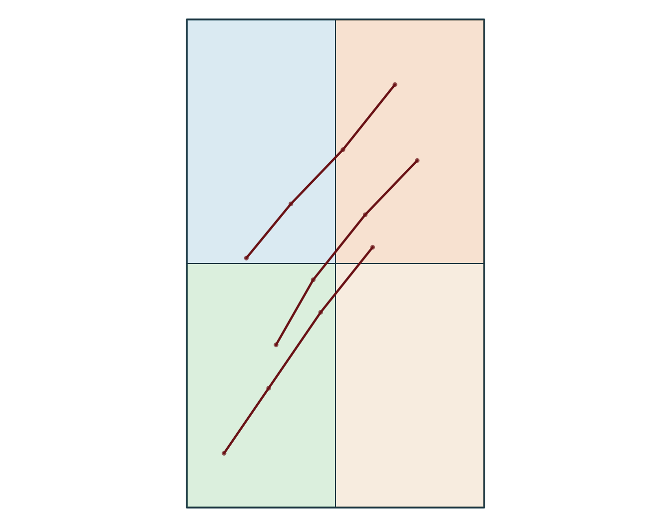
Cartographie statique rapide
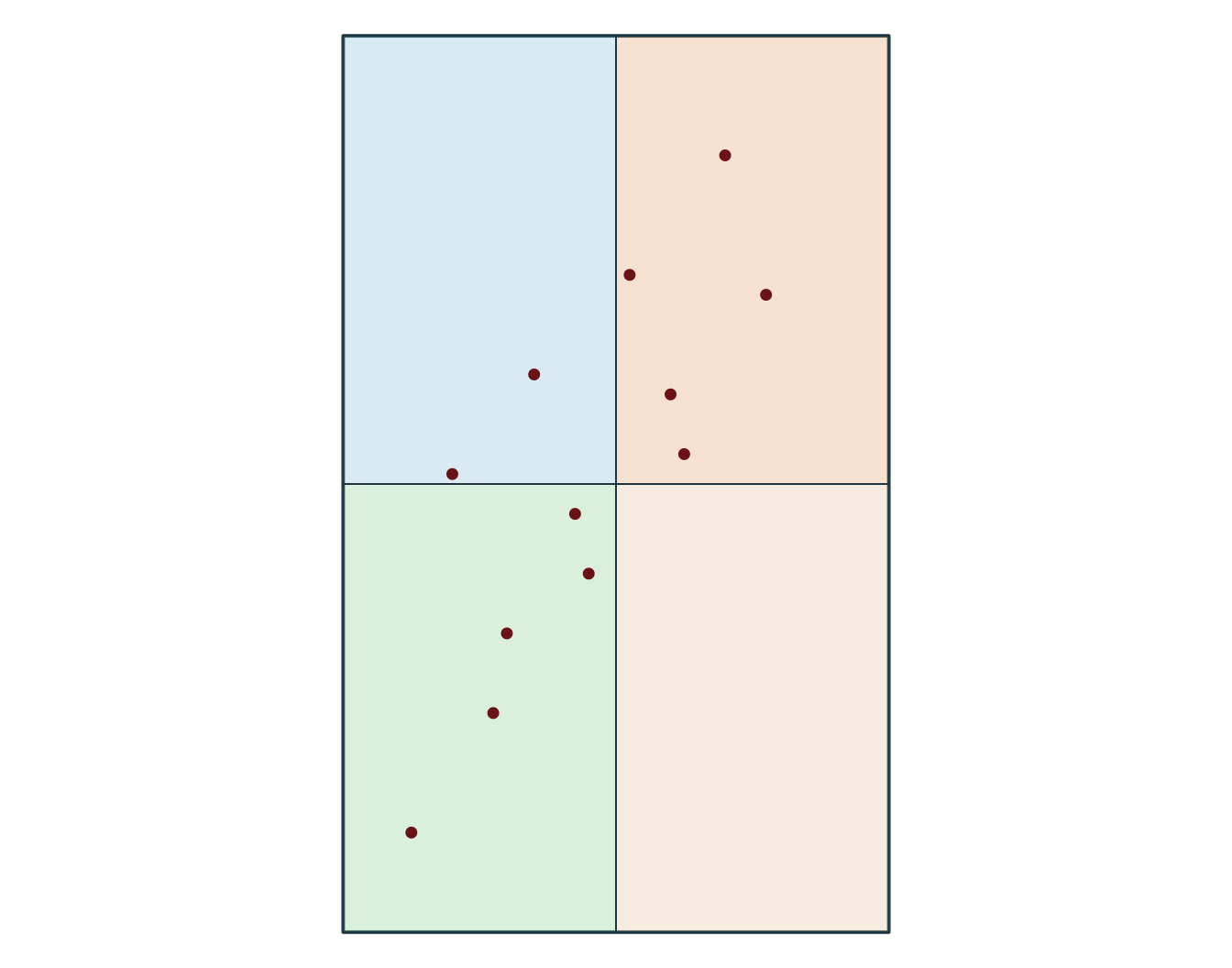

Filtrer vers une zone d’étude
Simple feature collection with 5 features and 8 fields
Geometry type: POINT
Dimension:     XY
Bounding box:  xmin: -72.79 ymin: 46.79 xmax: -72.69 ymax: 46.94
Geodetic CRS:  WGS 84
  obs_id track_id seq           timestamp    lon   lat category value
1  OBS03        A   3 2026-03-01 10:00:00 -72.79 46.88   forest    21
2  OBS04        A   4 2026-03-01 11:00:00 -72.72 46.94   forest    24
3  OBS07        B   3 2026-03-02 10:00:00 -72.76 46.82  wetland    17
4  OBS08        B   4 2026-03-02 11:00:00 -72.69 46.87  wetland    18
5  OBS12        C   4 2026-03-03 11:00:00 -72.75 46.79    urban    19
              geometry
1 POINT (-72.79 46.88)
2 POINT (-72.72 46.94)
3 POINT (-72.76 46.82)
4 POINT (-72.69 46.87)
5 POINT (-72.75 46.79)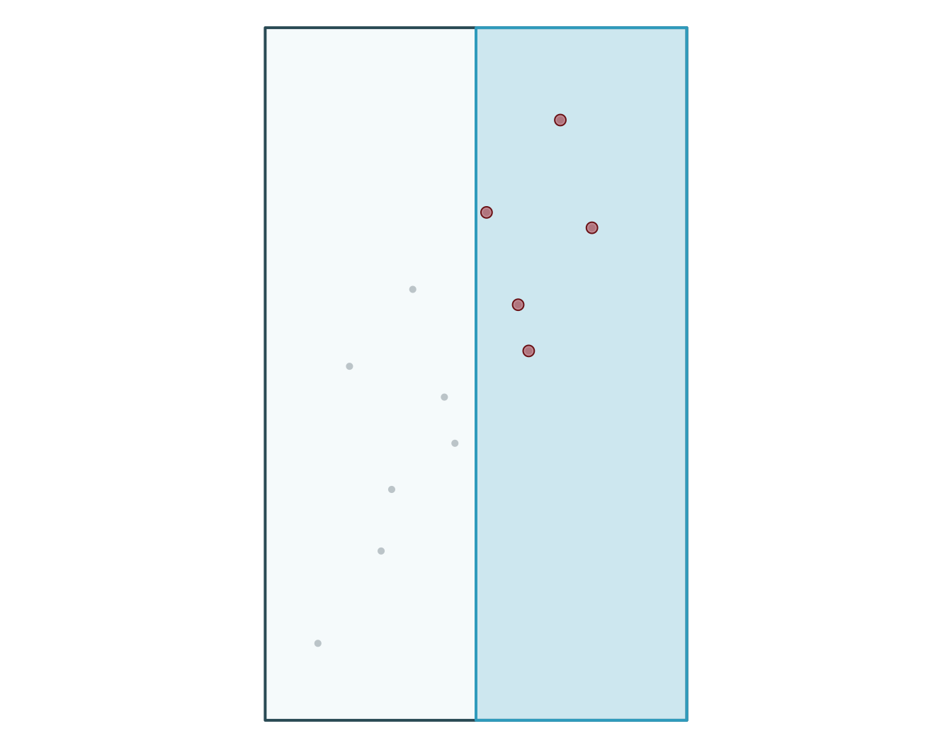
  obs_id track_id seq           timestamp category value
1  OBS03        A   3 2026-03-01 10:00:00   forest    21
2  OBS04        A   4 2026-03-01 11:00:00   forest    24
3  OBS07        B   3 2026-03-02 10:00:00  wetland    17
4  OBS08        B   4 2026-03-02 11:00:00  wetland    18
5  OBS12        C   4 2026-03-03 11:00:00    urban    19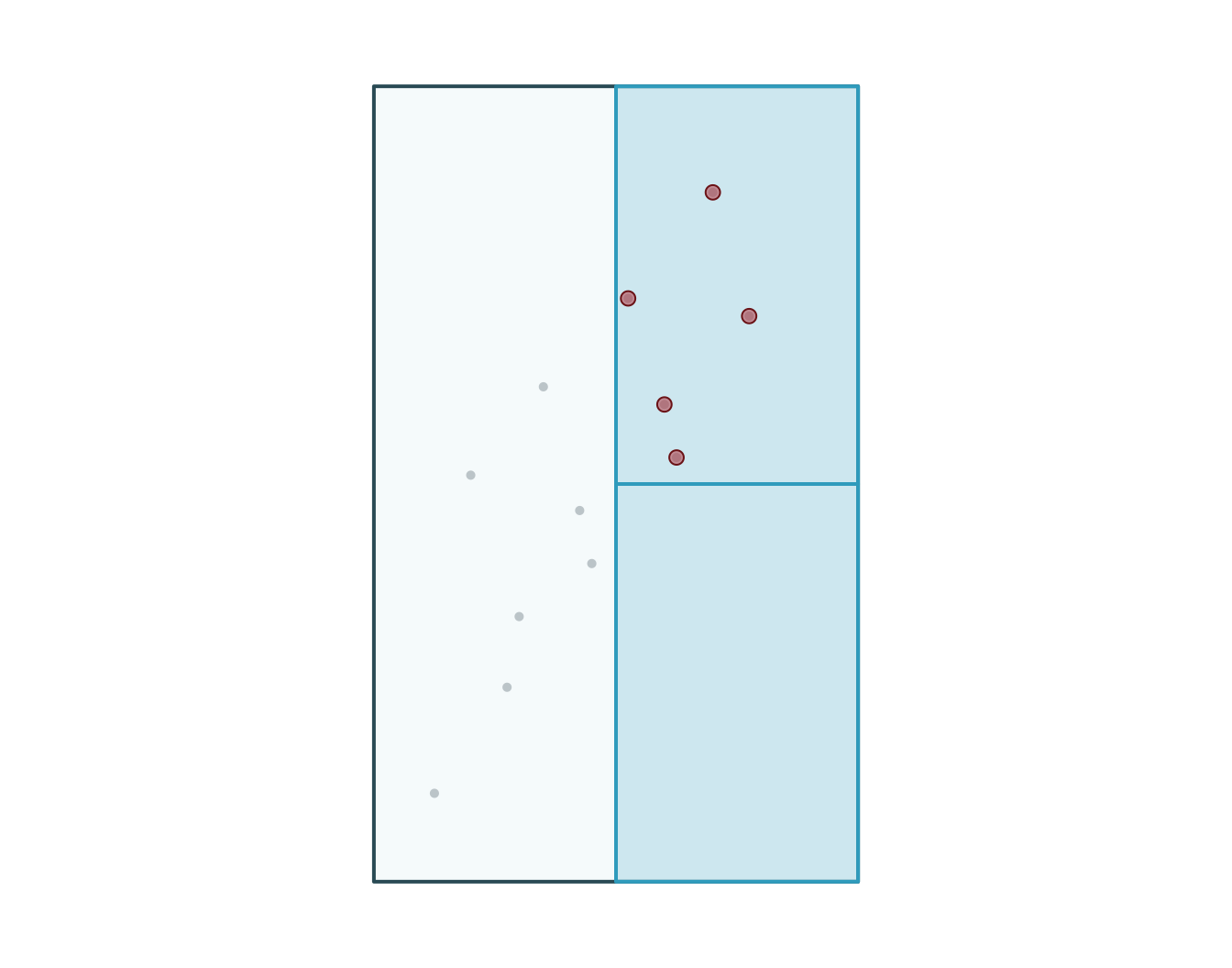
Joindre des attributs aux entités
  obs_id track_id seq           timestamp    lon   lat    category value
1  OBS01        A   1 2026-03-01 08:00:00 -72.92 46.78       urban    14
2  OBS02        A   2 2026-03-01 09:00:00 -72.86 46.83       urban    16
3  OBS03        A   3 2026-03-01 10:00:00 -72.79 46.88      forest    21
4  OBS04        A   4 2026-03-01 11:00:00 -72.72 46.94      forest    24
5  OBS05        B   1 2026-03-02 08:00:00 -72.88 46.70 agriculture    11
6  OBS06        B   2 2026-03-02 09:00:00 -72.83 46.76 agriculture    13
  zone_id zone_type
1      NW    forest
2      NW    forest
3      NE     urban
4      NE     urban
5      SW   wetland
6      SW   wetland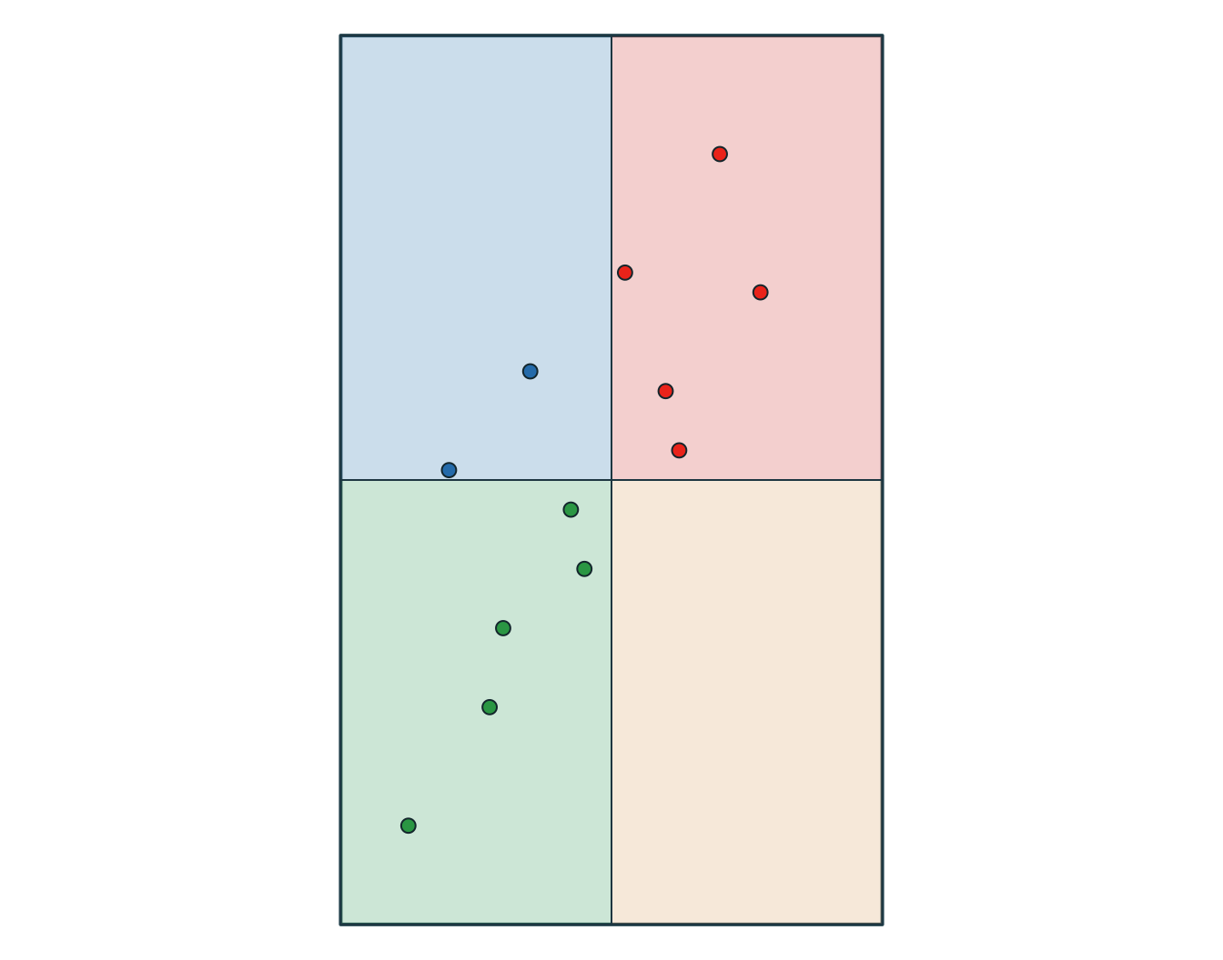
  obs_id track_id seq           timestamp    category value zone_id zone_type
1  OBS01        A   1 2026-03-01 08:00:00       urban    14      NW    forest
2  OBS02        A   2 2026-03-01 09:00:00       urban    16      NW    forest
3  OBS03        A   3 2026-03-01 10:00:00      forest    21      NE     urban
4  OBS04        A   4 2026-03-01 11:00:00      forest    24      NE     urban
5  OBS05        B   1 2026-03-02 08:00:00 agriculture    11      SW   wetland
6  OBS06        B   2 2026-03-02 09:00:00 agriculture    13      SW   wetland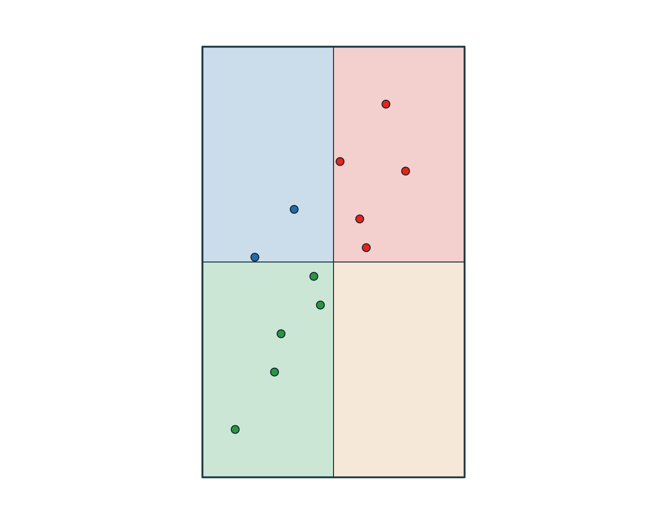
Intersecter les géométries
# A tibble: 6 × 3
  track_id zone_id zone_type
  <chr>    <chr>   <chr>
1 A        NW      forest
2 B        NW      forest
3 A        NE      urban
4 B        NE      urban
5 C        NE      urban
6 B SW wetland 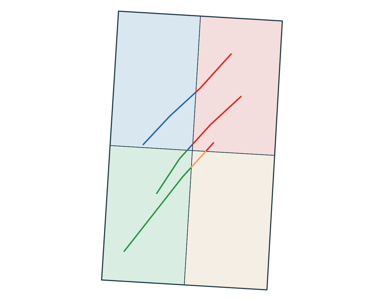
Zones tampon
[1] POLYGON
18 Levels: GEOMETRY POINT LINESTRING POLYGON MULTIPOINT ... TRIANGLE
obs_id track_id seq timestamp lon lat category value
1 OBS01 A 1 2026-03-01 08:00:00 -72.92 46.78 urban 14
2 OBS02 A 2 2026-03-01 09:00:00 -72.86 46.83 urban 16
3 OBS03 A 3 2026-03-01 10:00:00 -72.79 46.88 forest 21
4 OBS04 A 4 2026-03-01 11:00:00 -72.72 46.94 forest 24
5 OBS05 B 1 2026-03-02 08:00:00 -72.88 46.70 agriculture 11
6 OBS06 B 2 2026-03-02 09:00:00 -72.83 46.76 agriculture 13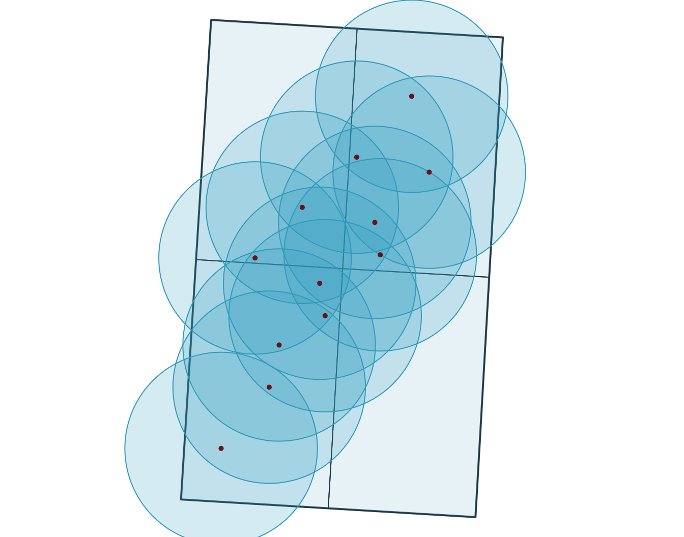
[1] "polygons" obs_id track_id seq timestamp category value
1 OBS01 A 1 2026-03-01 08:00:00 urban 14
2 OBS02 A 2 2026-03-01 09:00:00 urban 16
3 OBS03 A 3 2026-03-01 10:00:00 forest 21
4 OBS04 A 4 2026-03-01 11:00:00 forest 24
5 OBS05 B 1 2026-03-02 08:00:00 agriculture 11
6 OBS06 B 2 2026-03-02 09:00:00 agriculture 13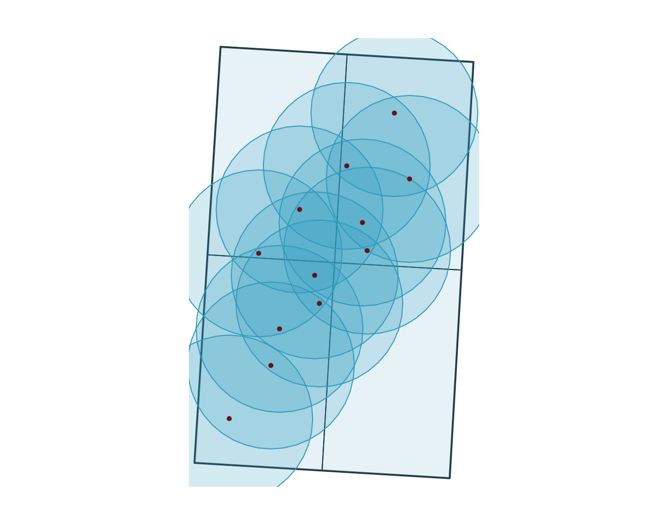
Lire des données raster
stars object with 2 dimensions and 1 attribute
attribute(s):
Min. 1st Qu. Median Mean 3rd Qu. Max.
surface.tif 9.6 40.8325 48.5 50.00007 59.805 100.32
dimension(s):
from to offset delta refsys point x/y
x 1 40 -73 0.01 WGS 84 FALSE [x]
y 1 40 47 -0.01125 WGS 84 FALSE [y]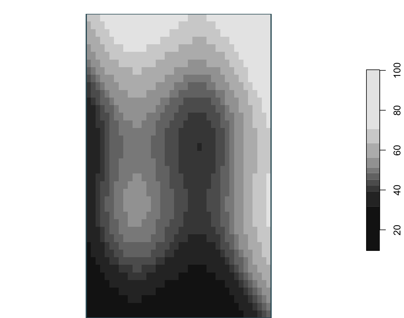
class : SpatRaster
size : 40, 40, 1 (nrow, ncol, nlyr)
resolution : 0.01, 0.01125 (x, y)
extent : -73, -72.6, 46.55, 47 (xmin, xmax, ymin, ymax)
coord. ref. : lon/lat WGS 84 (EPSG:4326)
source : surface.tif
name : surface_value
min value : 9.60
max value : 100.32 
Visualisation statique de rasters
Découper, masquer, projeter
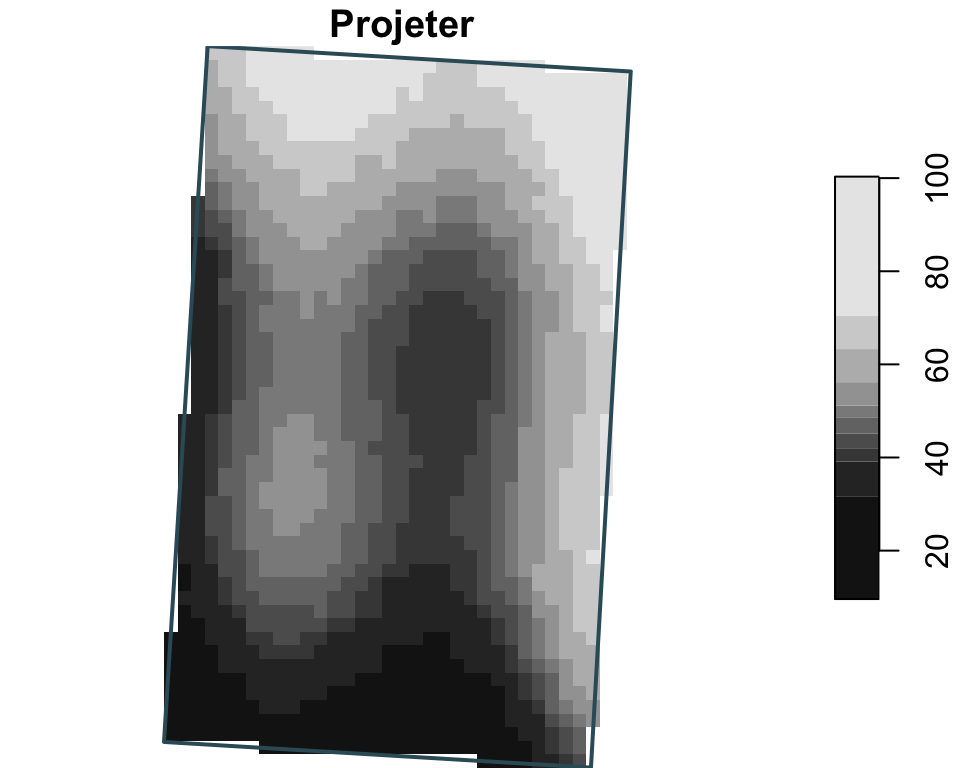
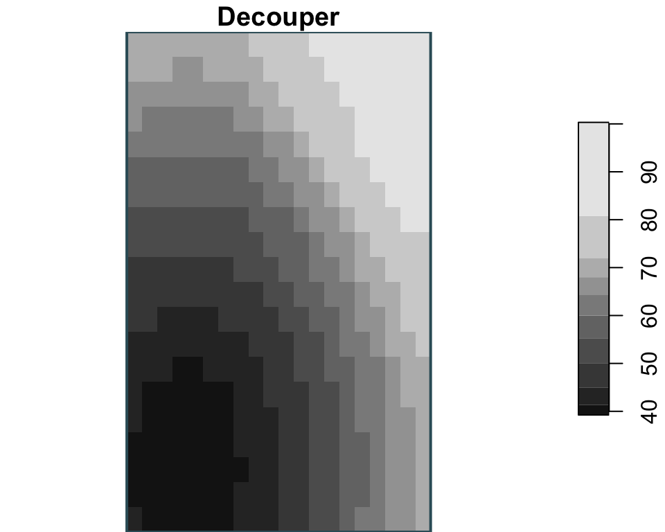
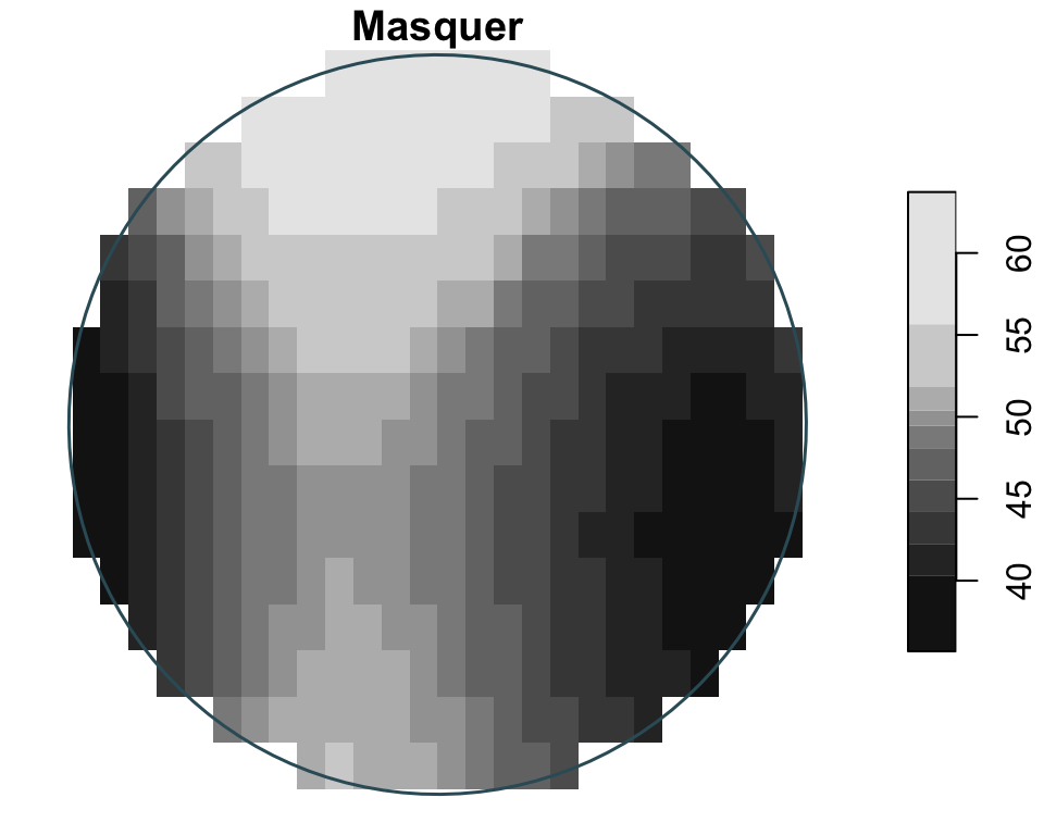
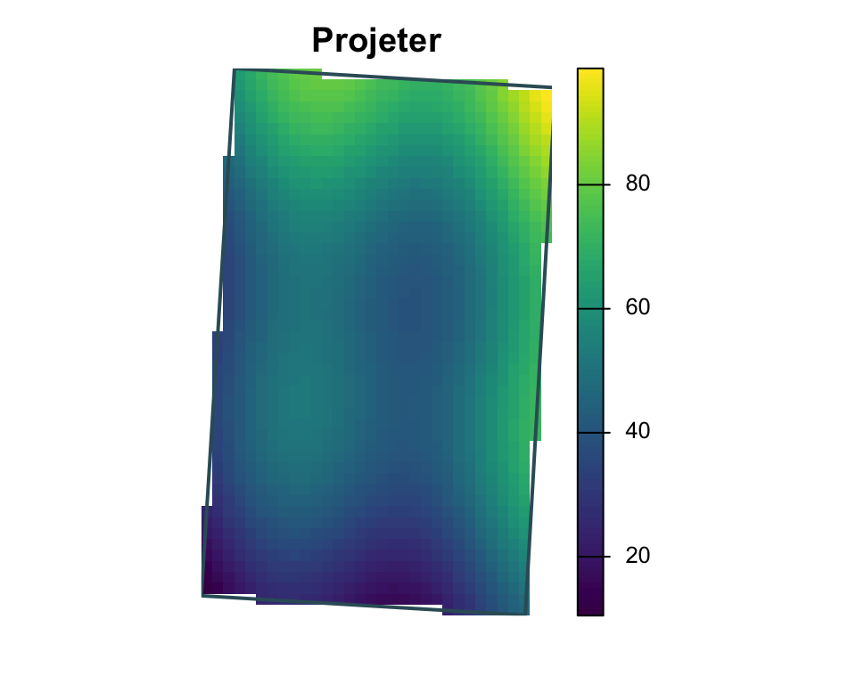
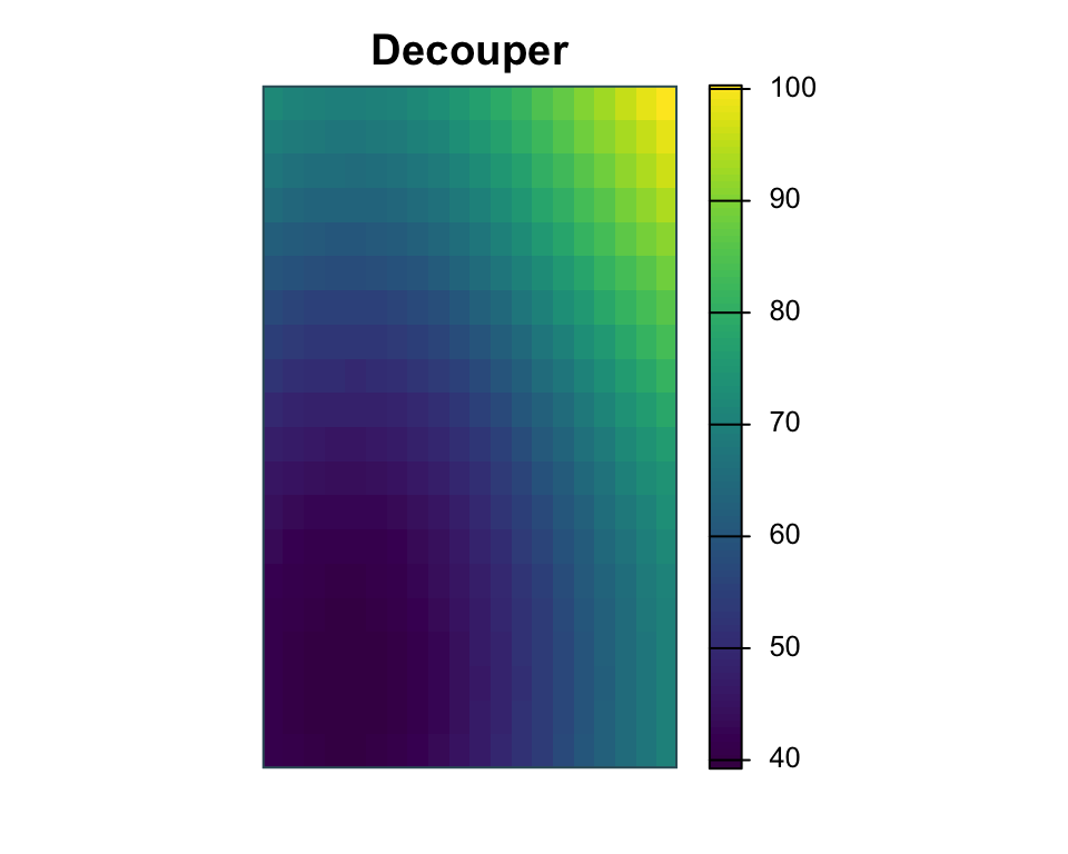
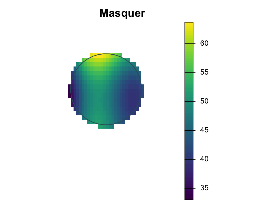
Manipulations raster
Ici les trois opérations sont présentées indépendamment : project change le CRS, crop utilisé une zone comme étendue cible, et mask conserve les cellules uniquement à l’intérieur d’une géométrie tampon.
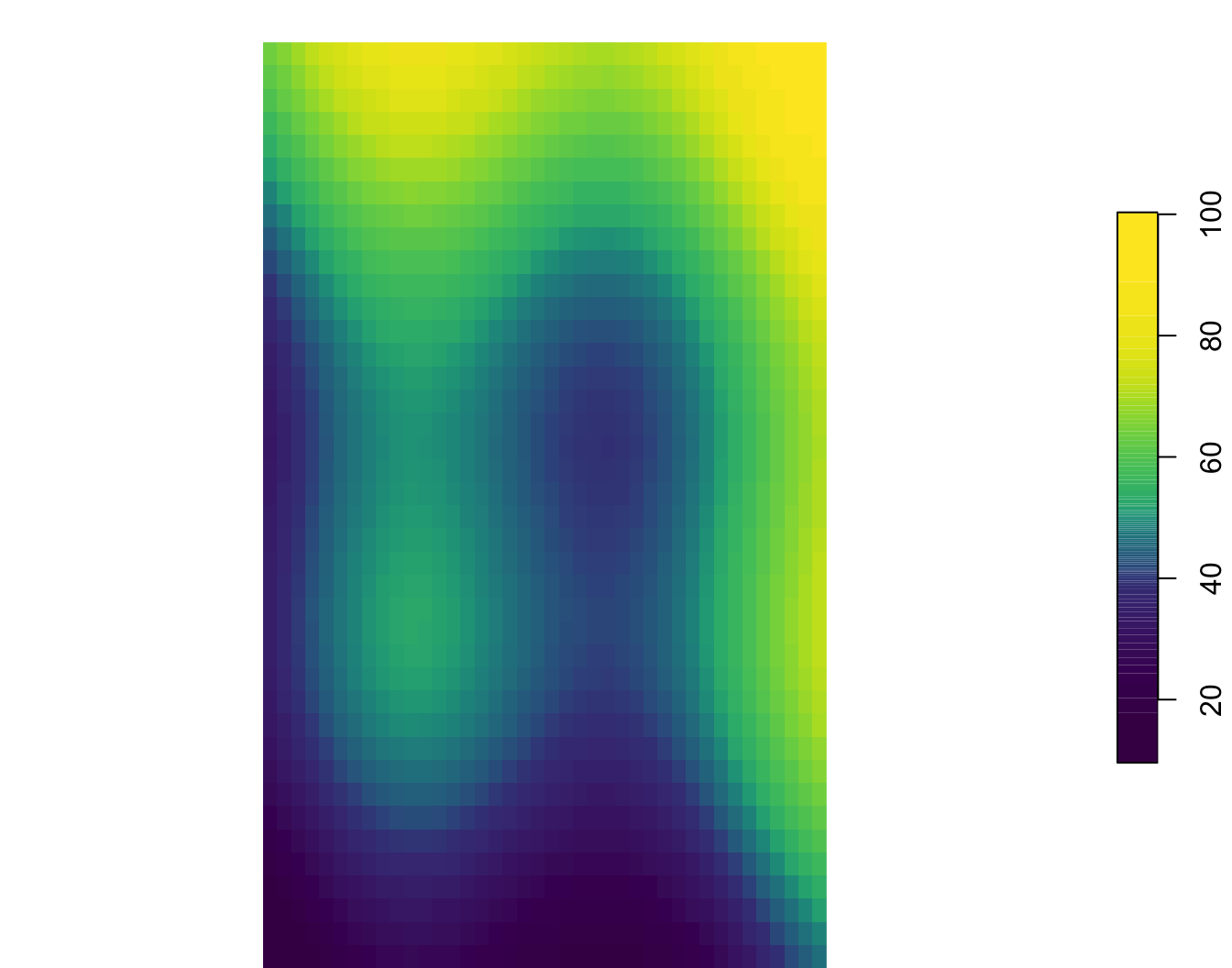
Rééchantillonnage
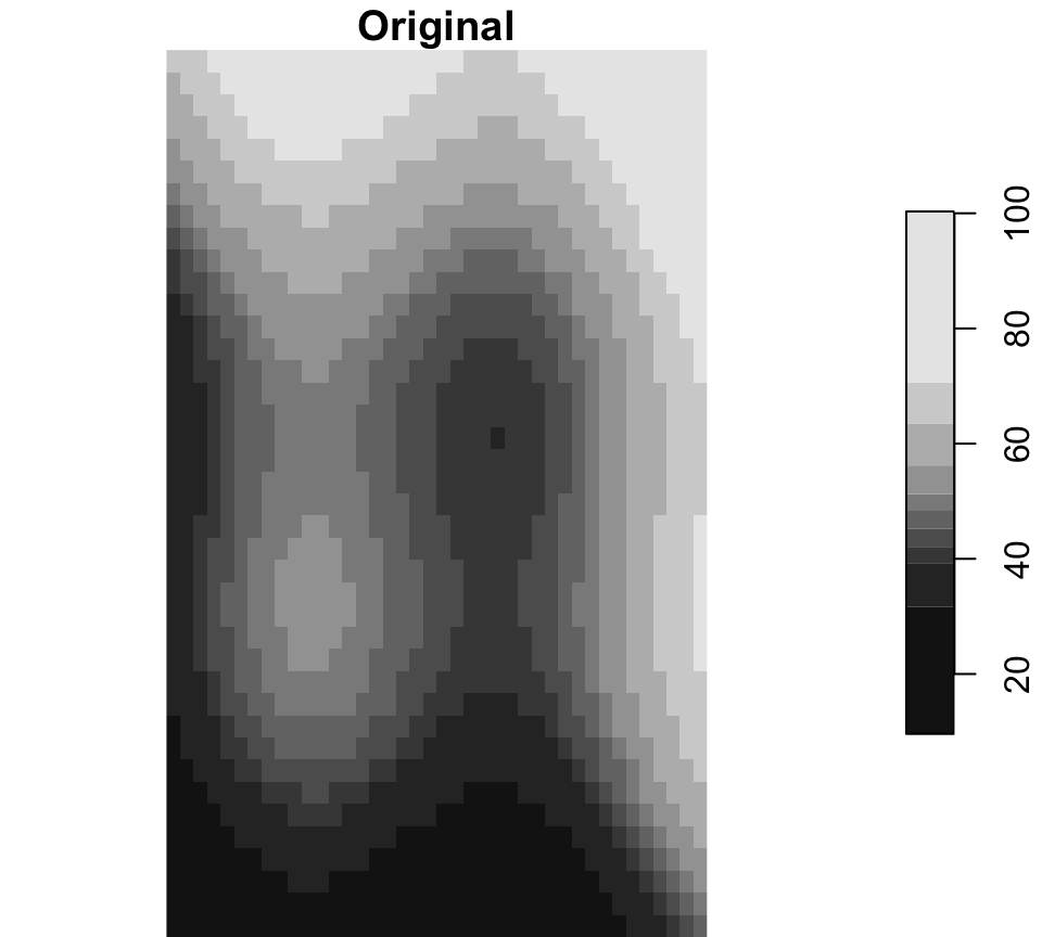
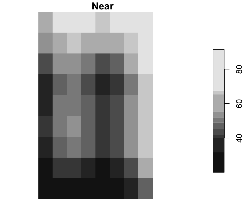
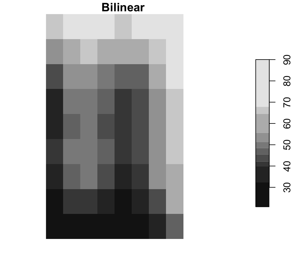
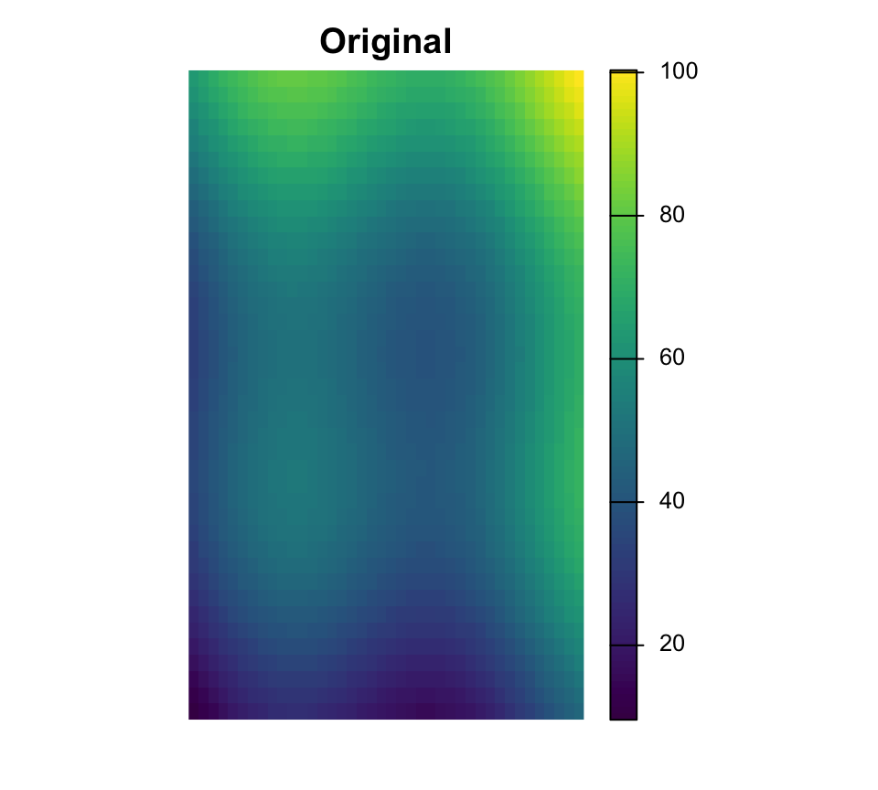
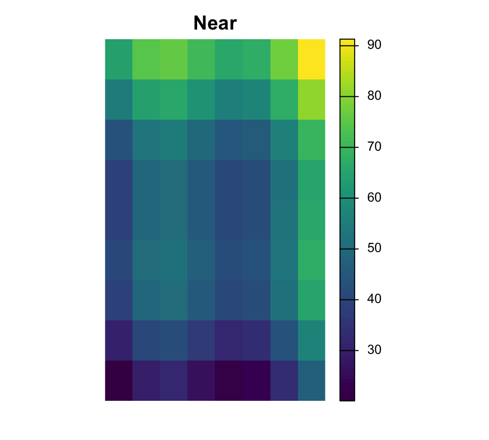
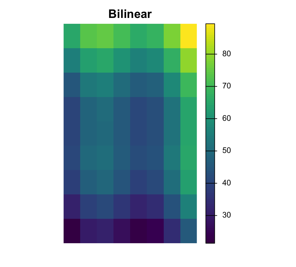
Le rééchantillonnage modifie la grille de cellules
Near est courant pour les rasters categoriques, tandis que bilinear est courant pour les surfaces continues.
Couches raster multiples
[1] "surface.tif" "surface_alt"[1] 2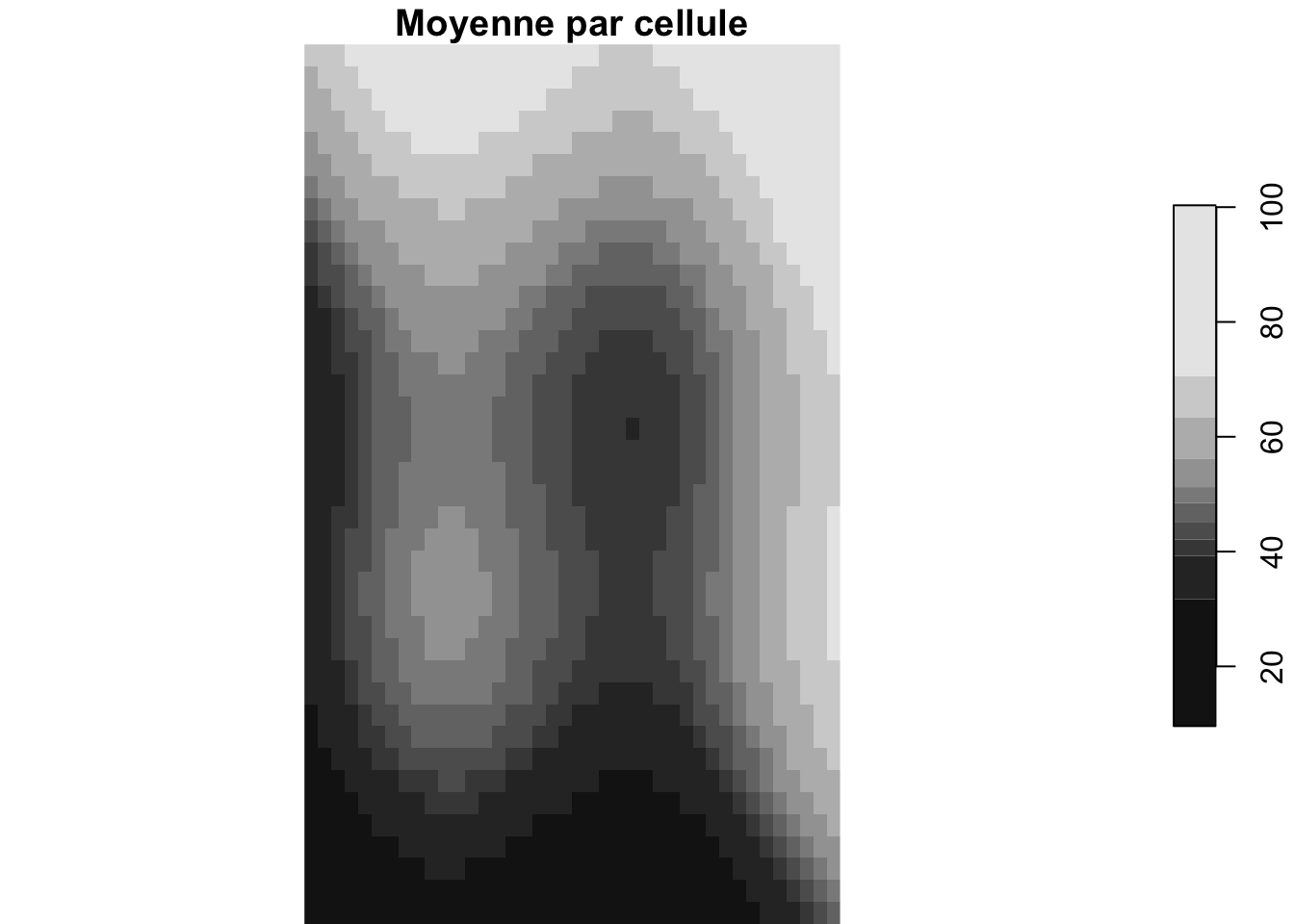
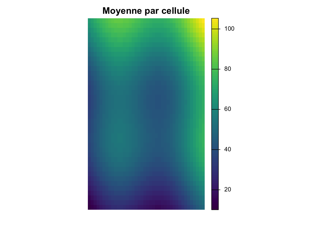
Rasters multi-couches
Peuvent représenter des bandes, variables ou pas de temps. Les fonctions par cellule combinent l’information à travers les couches.
Travailler avec vecteurs et rasters

Extraction raster par points
  obs_id track_id seq           timestamp    lon   lat    category value
1  OBS01        A   1 2026-03-01 08:00:00 -72.92 46.78       urban    14
2  OBS02        A   2 2026-03-01 09:00:00 -72.86 46.83       urban    16
3  OBS03        A   3 2026-03-01 10:00:00 -72.79 46.88      forest    21
4  OBS04        A   4 2026-03-01 11:00:00 -72.72 46.94      forest    24
5  OBS05        B   1 2026-03-02 08:00:00 -72.88 46.70 agriculture    11
6  OBS06        B   2 2026-03-02 09:00:00 -72.83 46.76 agriculture    13
zone_id zone_type surface_value
1 NW forest 49.71
2 NW forest 48.70
3 NE urban 47.72
4 NE urban 61.39
5 SW wetland 51.67
6 SW wetland 45.88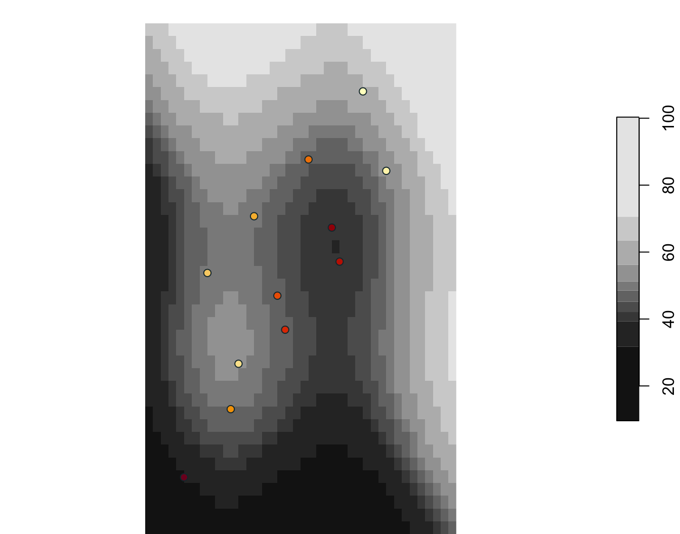
  obs_id zone_id zone_type surface_value
1  OBS01      NW    forest         48.69
2  OBS02      NW    forest         49.60
3  OBS03      NE     urban         47.72
4  OBS04      NE     urban         59.98
5  OBS05      SW   wetland         51.67
6  OBS06      SW   wetland         47.16
Extraction raster par lignes
# A tibble: 3 × 2
  track_id surface_value
  <chr>            <dbl>
1 A                 50.0
2 B                 45.0
3 C                 44.2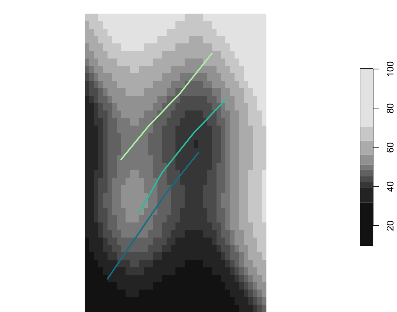
Extraction raster par polygones
  zone_id   zone_type surface_value
1      NW      forest      55.93852
2      NE       urban      60.33677
3      SW     wetland      39.66305
4      SE agriculture      44.06193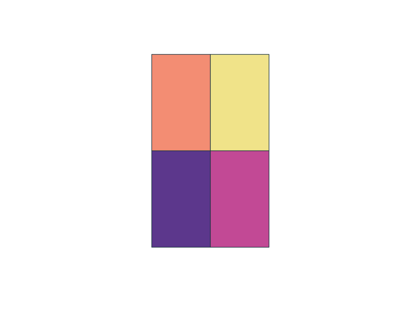
Bonus : GLM avancé
pseudo_points <- st_sample(aoi_qc, size = nrow(points_qc), exact = TRUE) |>
  st_as_sf() |>
  st_join(zones_qc[, c("zone_id", "zone_type")])

pseudo_points$surface_value <- st_extract(surface_qc, pseudo_points)[[1]]
pseudo_points$presence <- 0
points_qc$presence <- 1

pa_data <- bind_rows(points_qc, pseudo_points) |>
  st_drop_geometry() |>
  filter(!is.na(zone_id), !is.na(surface_value))

glm_pa <- glm(presence ~ surface_value + zone_type, family = binomial(), data = pa_data)
term Estimate Std..Error z.value Pr...z..
1 (Intercept) -16.407 3143.229 -0.005 0.996
2 surface_value -0.039 0.036 -1.098 0.272
3 zone_typeforest 19.471 3143.229 0.006 0.995
4 zone_typeurban 18.584 3143.229 0.006 0.995
5 zone_typewetland 18.917 3143.229 0.006 0.995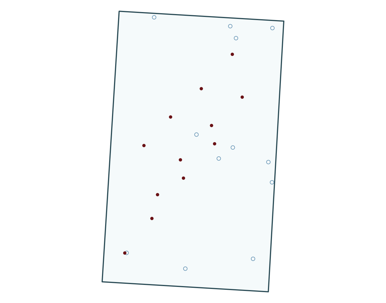
pseudo_points <- spatSample(aoi_qc, size = nrow(points_qc), method = "random", as.points = TRUE)
pseudo_zone <- extract(zones_qc, pseudo_points)
pseudo_surface <- extract(surface_qc, pseudo_points)
pseudo_points <- cbind(pseudo_points, pseudo_zone[, c("zone_id", "zone_type")], pseudo_surface[, "surface_value", drop = FALSE])
pseudo_points$presence <- 0
points_qc$presence <- 1

pa_data <- bind_rows(as.data.frame(points_qc), as.data.frame(pseudo_points)) |>
  filter(!is.na(zone_id), !is.na(surface_value))

glm_pa <- glm(presence ~ surface_value + zone_type, family = binomial(), data = pa_data)
term Estimate Std..Error z.value Pr...z..
1 (Intercept) -13.913 2782.290 -0.005 0.996
2 surface_value -0.061 0.062 -0.981 0.326
3 zone_typeforest 16.642 2782.287 0.006 0.995
4 zone_typeurban 17.569 2782.287 0.006 0.995
5 zone_typewetland 17.009 2782.287 0.006 0.995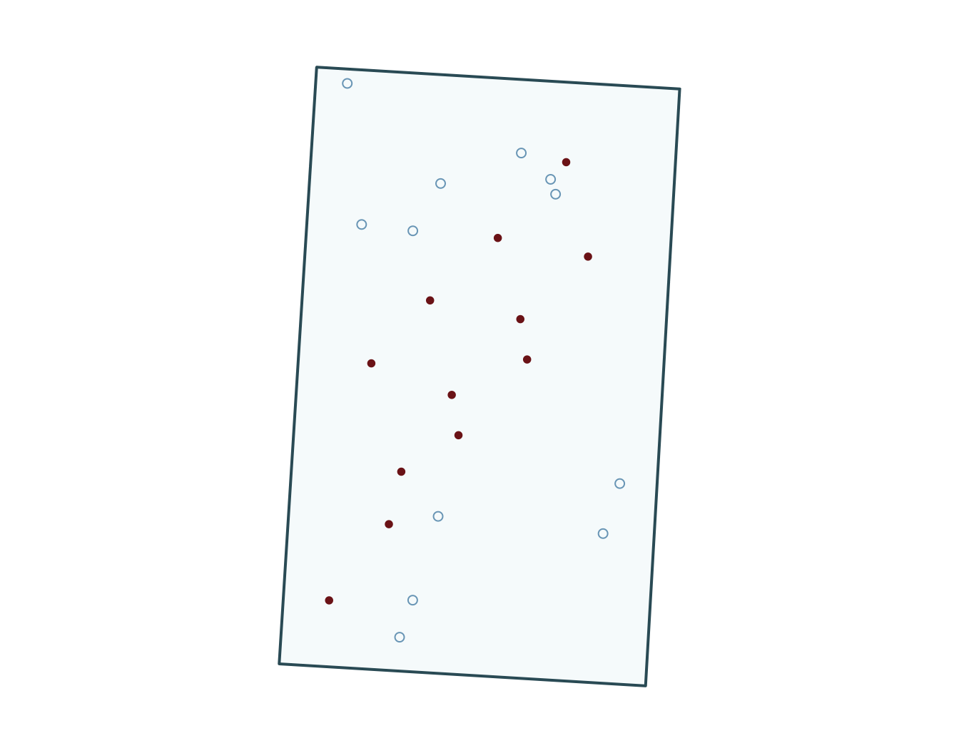
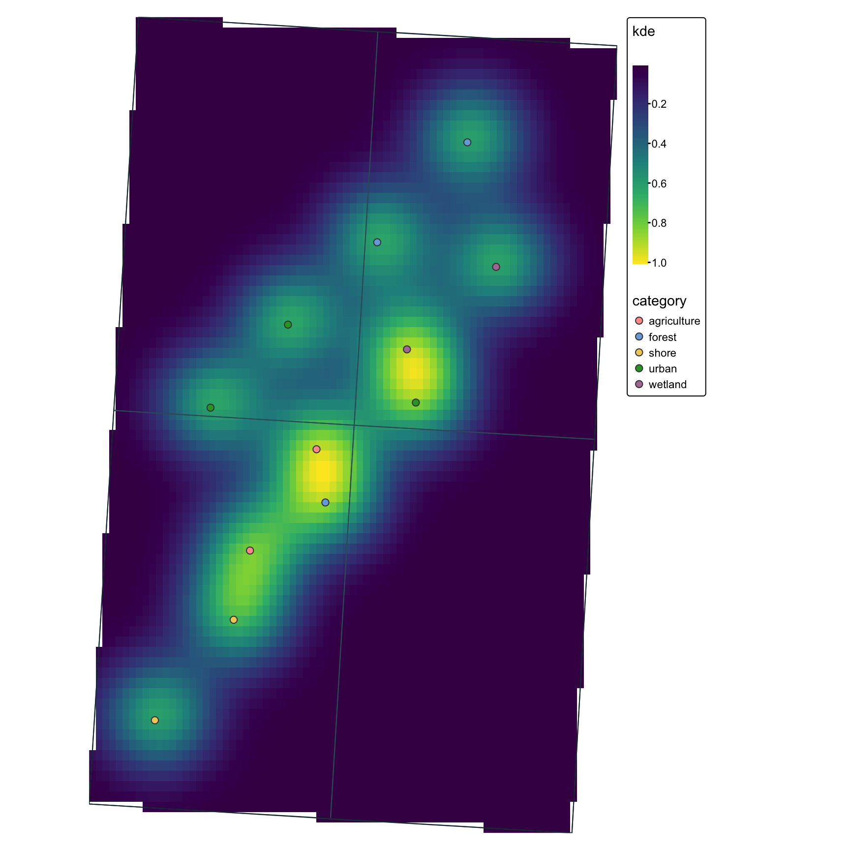
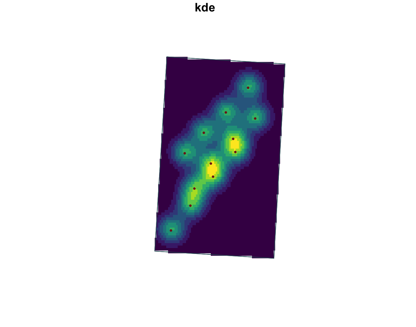
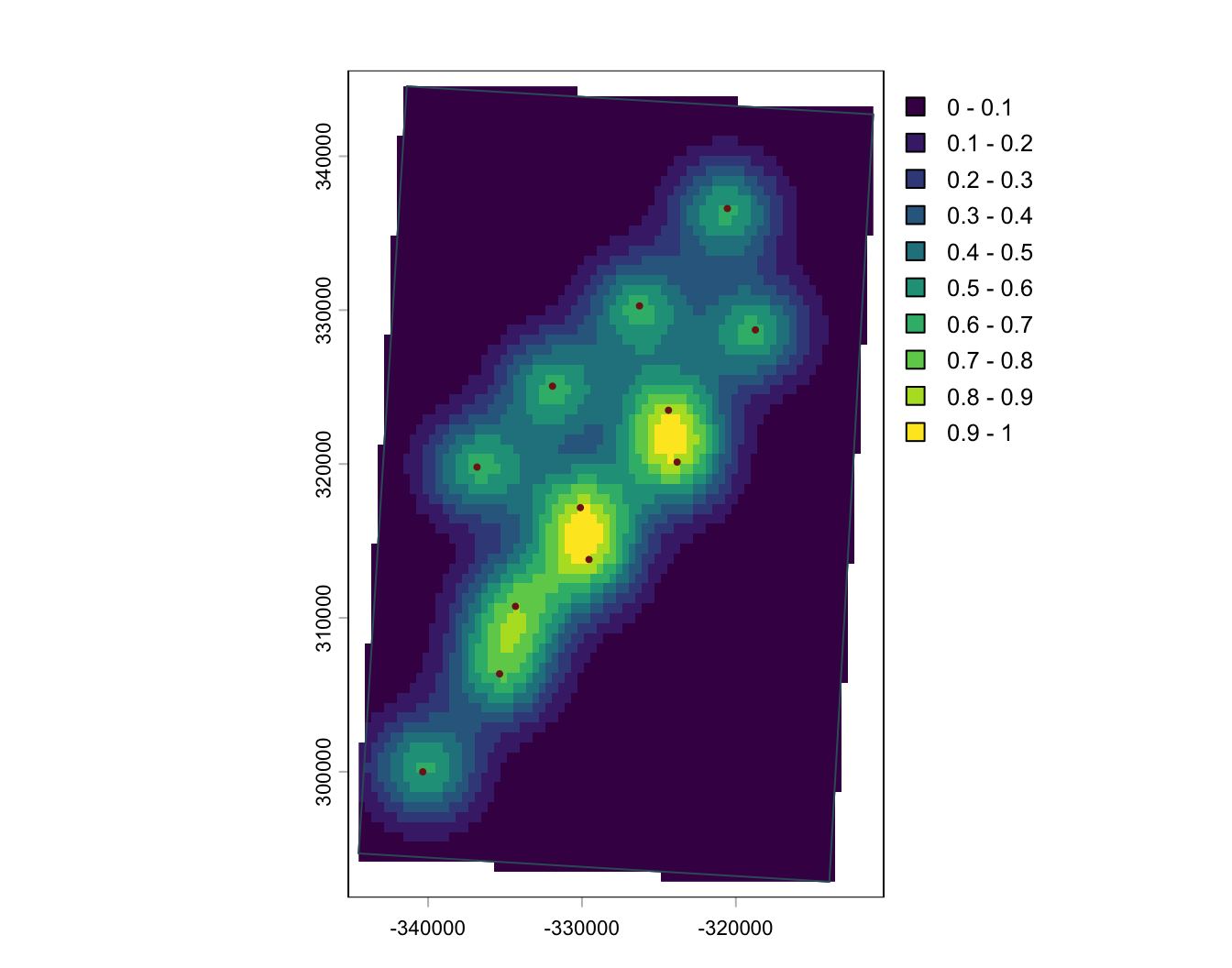
Estimation de densité (KDE)
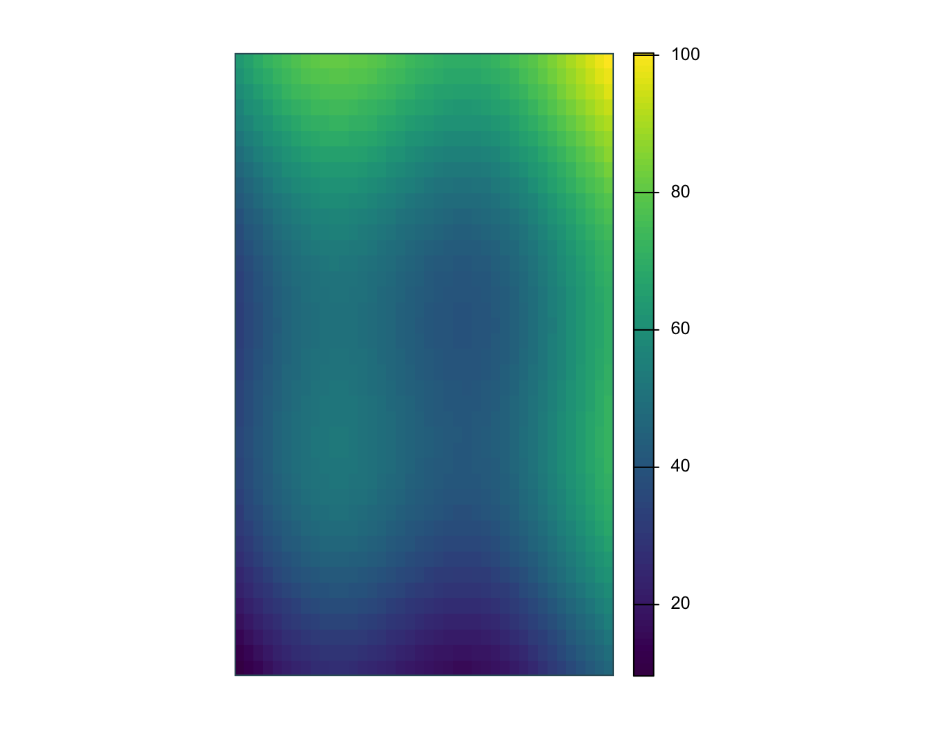
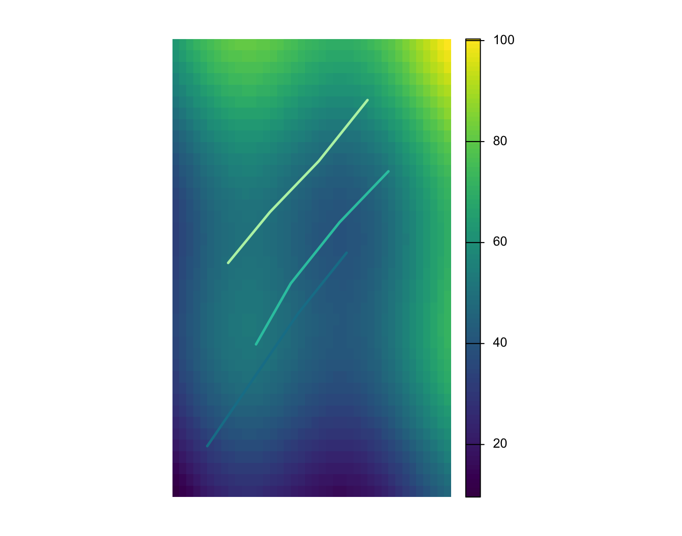
Cartographie avancee avec ggplot2
ggplot2 fonctionne particulièrement bien pour des cartes statiques soignées, notamment avec les objets sf et stars.
gg <- ggplot() +
  geom_stars(
    data = points_kde_sf_plot
  ) +
  scale_fill_viridis_c(name = "KDE") +
  geom_sf(
    data = zones_qc,
    fill = NA,
    color = "#355c67"
  ) +
  geom_sf(
    data = aoi_qc,
    fill = NA,
    color = "#17313b"
  ) +
  geom_sf(
    data = points_sf_qc,
    aes(color = category),
    size = 1.7
   ) +
  coord_sf(expand = FALSE) +
  theme_minimal()
gg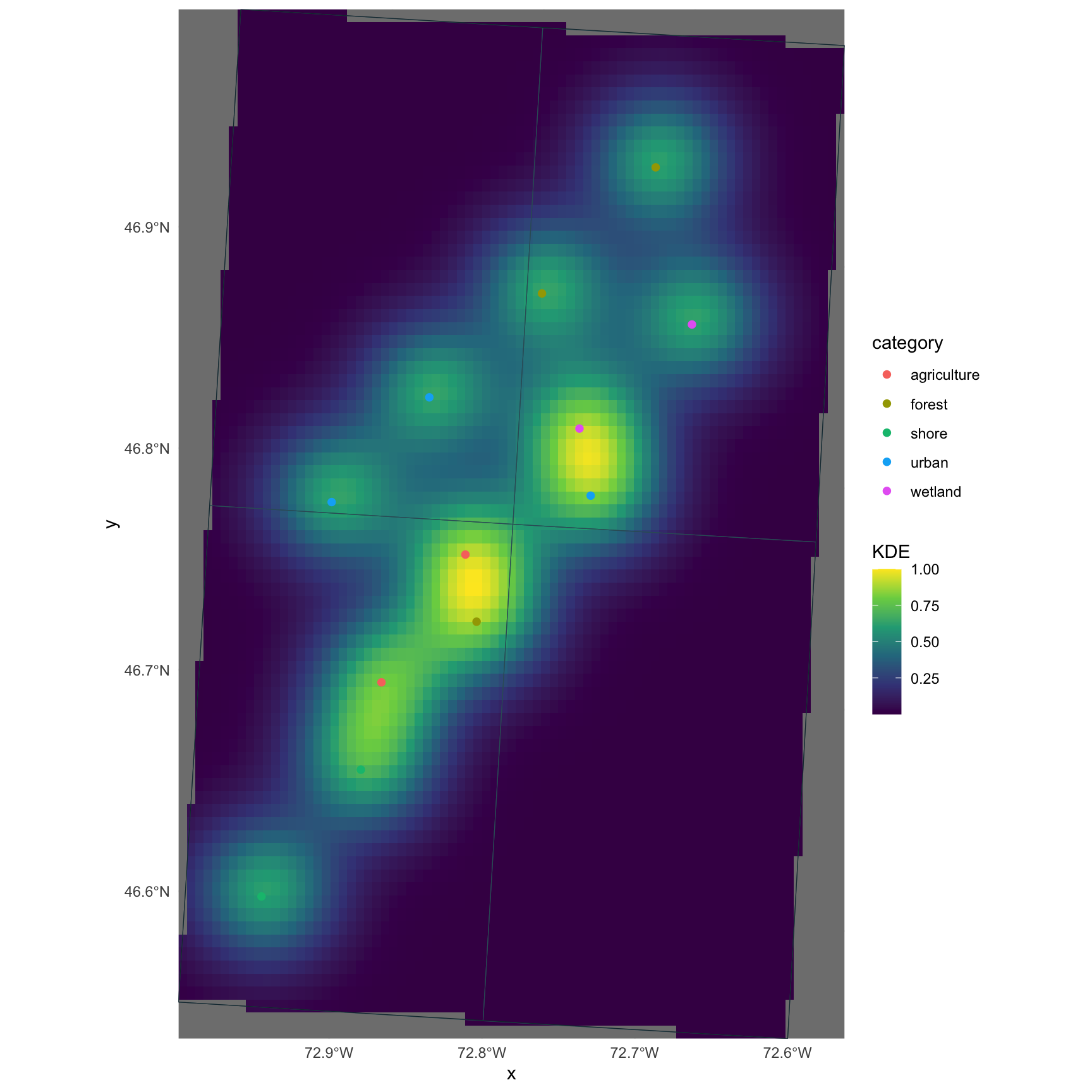
Cartographie avancee avec tmap
tmap est concu pour la cartographie thématique et fonctionne bien quand vous souhaitez une grammaire plus orientée cartographie que ggplot2.
tm <- tm_shape(points_kde_sf_plot) +
  tm_raster(col.scale = tm_scale_continuous(
    values = "viridis"
  )) +
  tm_shape(zones_qc) +
  tm_borders(col = "#355c67") +
  tm_shape(points_sf_qc) +
  tm_symbols(
    fill = "category",
    size = 0.5
  ) +
  tm_shape(aoi_qc) +
  tm_borders(col = "#17313b") +
  tm_layout(
    frame = FALSE,
    legend.outside = TRUE
  )
tm