Main Spatial R Packages
New ecosystem
Old ecosystem
2026-03-25
| Object type | Description |
sf
|
stars
|
terra
|
|---|---|---|---|---|
| Vector | Where are the features? | |||
 Points Points
|
Discrete locations with coordinates and attributes. | ✓ | ✓ | |
 Lines Lines
|
Linear features such as roads, rivers, or tracks. | ✓ | ✓ | |
 Polygons Polygons
|
Areas such as lakes, study zones, or administrative boundaries. | ✓ | ✓ | |
| Raster | What is the value across space? | |||
 Rasters Rasters
|
Gridded surfaces with values stored in cells. | ✓ | ✓ |
Choose Your Route
Do both levels!
More advanced participants can complete both workflows, as there will be advanced workflows available with both points and lines.
Simple feature collection with 1 feature and 1 field
Geometry type: POLYGON
Dimension: XY
Bounding box: xmin: -73 ymin: 46.55 xmax: -72.6 ymax: 47
Geodetic CRS: WGS 84
name geom
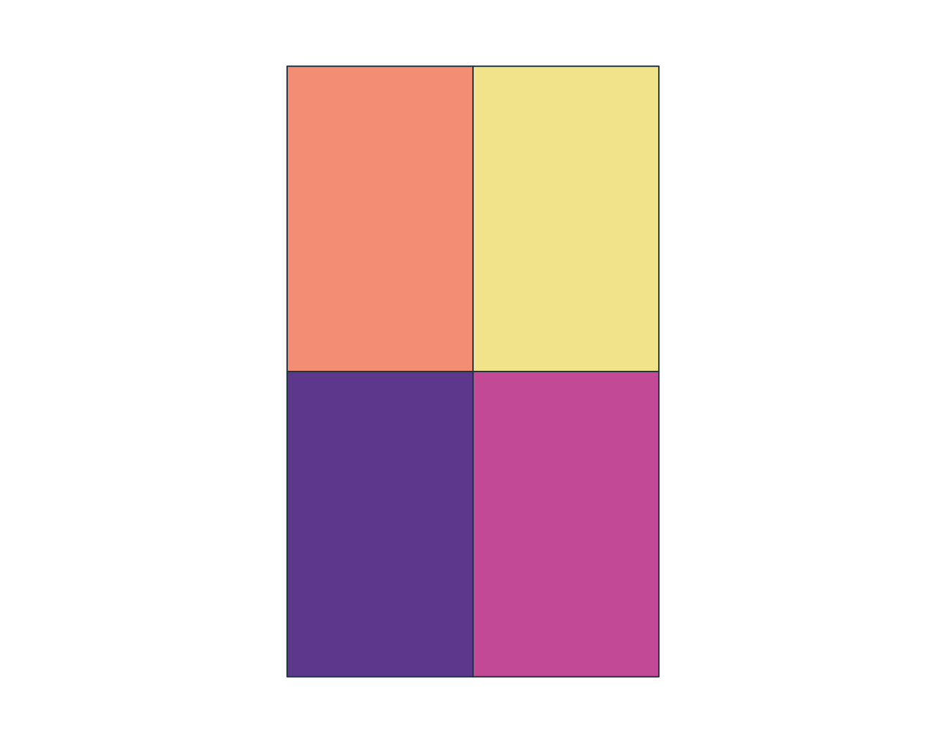
1 study_area POLYGON ((-73 46.55, -72.6 ...Simple feature collection with 4 features and 2 fields
Geometry type: POLYGON
Dimension: XY
Bounding box: xmin: -73 ymin: 46.55 xmax: -72.6 ymax: 47
Geodetic CRS: WGS 84
zone_id zone_type geom
1 NW forest POLYGON ((-73 46.775, -72.8...
2 NE urban POLYGON ((-72.8 46.775, -72...
3 SW wetland POLYGON ((-73 46.55, -72.8 ...
4 SE agriculture POLYGON ((-72.8 46.55, -72....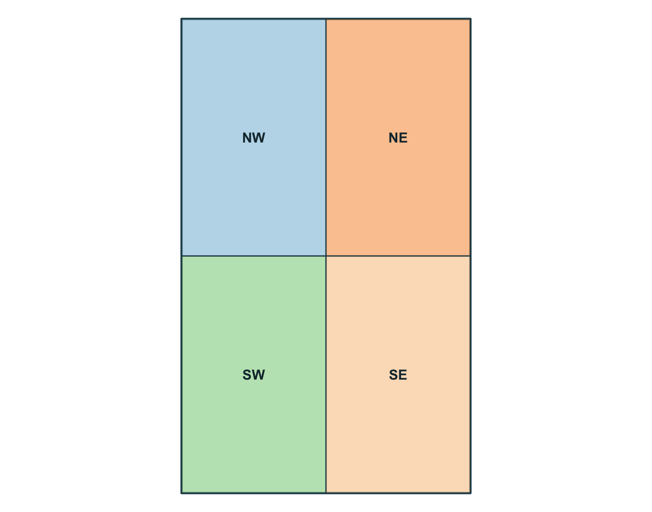
Simple feature collection with 6 features and 8 fields
Geometry type: POINT
Dimension:     XY
Bounding box:  xmin: -72.92 ymin: 46.7 xmax: -72.72 ymax: 46.94
Geodetic CRS:  WGS 84
  obs_id track_id seq           timestamp    lon   lat    category value
1  OBS01        A   1 2026-03-01 08:00:00 -72.92 46.78       urban    14
2  OBS02        A   2 2026-03-01 09:00:00 -72.86 46.83       urban    16
3  OBS03        A   3 2026-03-01 10:00:00 -72.79 46.88      forest    21
4  OBS04        A   4 2026-03-01 11:00:00 -72.72 46.94      forest    24
5  OBS05        B   1 2026-03-02 08:00:00 -72.88 46.70 agriculture    11
6  OBS06        B   2 2026-03-02 09:00:00 -72.83 46.76 agriculture    13
              geometry
1 POINT (-72.92 46.78)
2 POINT (-72.86 46.83)
3 POINT (-72.79 46.88)
4 POINT (-72.72 46.94)
5  POINT (-72.88 46.7)
6 POINT (-72.83 46.76)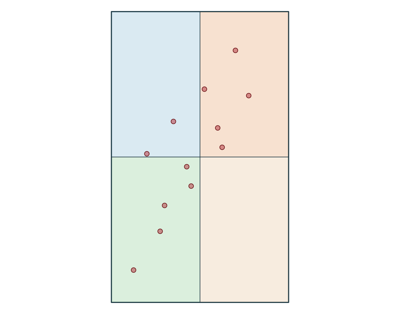
  obs_id track_id seq           timestamp    category value
1  OBS01        A   1 2026-03-01 08:00:00       urban    14
2  OBS02        A   2 2026-03-01 09:00:00       urban    16
3  OBS03        A   3 2026-03-01 10:00:00      forest    21
4  OBS04        A   4 2026-03-01 11:00:00      forest    24
5  OBS05        B   1 2026-03-02 08:00:00 agriculture    11
6  OBS06        B   2 2026-03-02 09:00:00 agriculture    13
[1] "EPSG:32198" xmin ymin xmax ymax
-340347.4 299996.5 -318731.5 336605.7 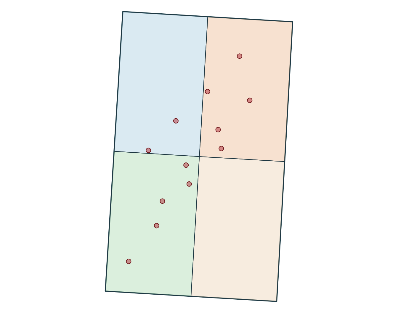
[1] "+proj=lcc +lat_0=44 +lon_0=-68.5 +lat_1=60 +lat_2=46 +x_0=0 +y_0=0 +datum=NAD83 +units=m +no_defs"SpatExtent : -340347.355525386, -318731.482880504, 299996.469057655, 336605.697992394 (xmin, xmax, ymin, ymax)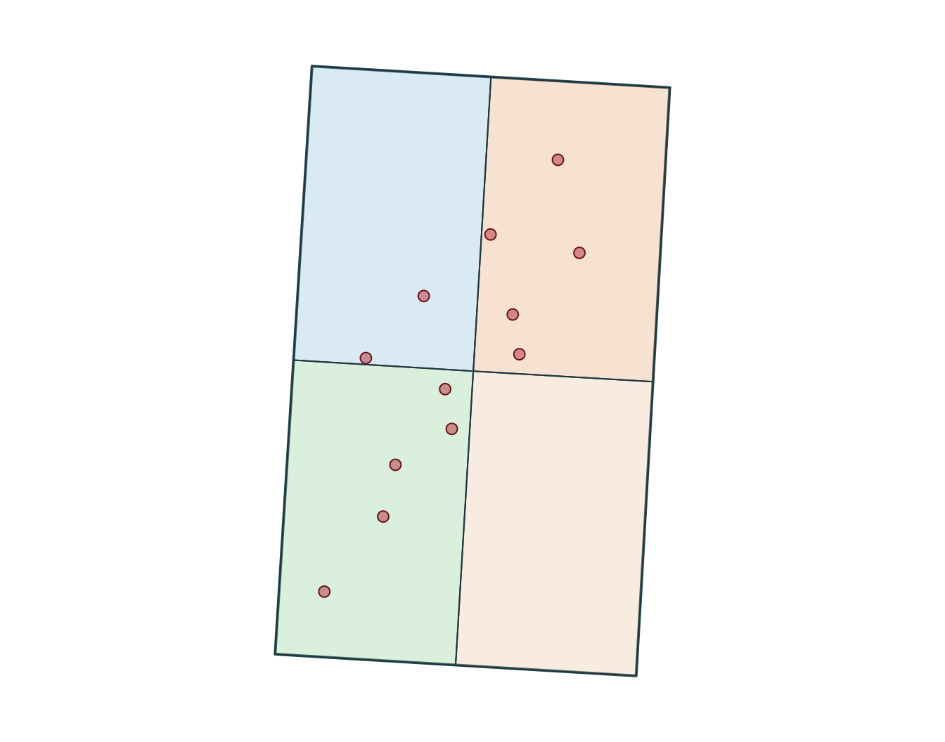
Measurements
Use a suitable projected CRS when you need interpretable distances, lengths, or areas.
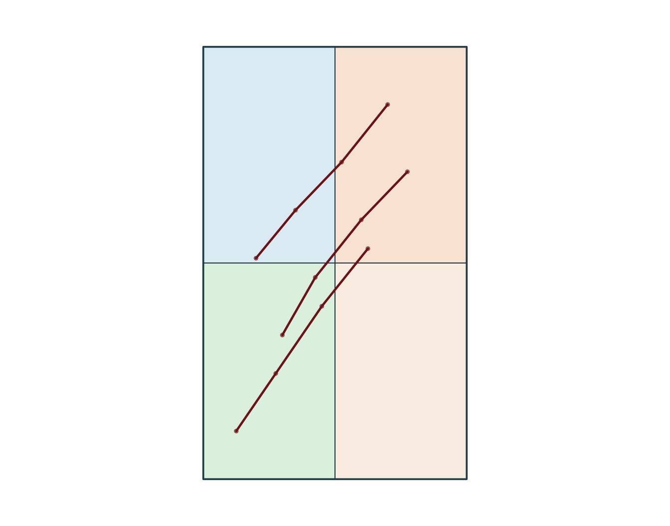
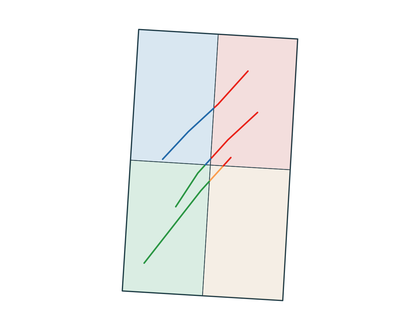
Simple feature collection with 3 features and 1 field
Geometry type: LINESTRING
Dimension:     XY
Bounding box:  xmin: -72.95 ymin: 46.6 xmax: -72.69 ymax: 46.94
Geodetic CRS:  WGS 84
# A tibble: 3 × 2
  track_id                                                 geometry
  <chr>                                            <LINESTRING [°]>
1 A        (-72.92 46.78, -72.86 46.83, -72.79 46.88, -72.72 46.94)
2 B         (-72.88 46.7, -72.83 46.76, -72.76 46.82, -72.69 46.87)
3 C         (-72.95 46.6, -72.89 46.66, -72.82 46.73, -72.75 46.79)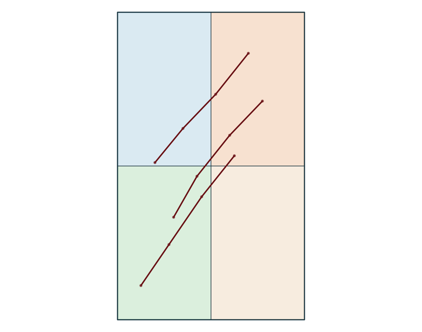
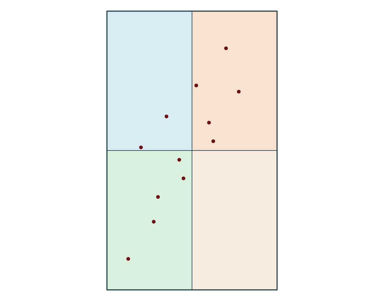
Simple feature collection with 5 features and 8 fields
Geometry type: POINT
Dimension:     XY
Bounding box:  xmin: -72.79 ymin: 46.79 xmax: -72.69 ymax: 46.94
Geodetic CRS:  WGS 84
  obs_id track_id seq           timestamp    lon   lat category value
1  OBS03        A   3 2026-03-01 10:00:00 -72.79 46.88   forest    21
2  OBS04        A   4 2026-03-01 11:00:00 -72.72 46.94   forest    24
3  OBS07        B   3 2026-03-02 10:00:00 -72.76 46.82  wetland    17
4  OBS08        B   4 2026-03-02 11:00:00 -72.69 46.87  wetland    18
5  OBS12        C   4 2026-03-03 11:00:00 -72.75 46.79    urban    19
              geometry
1 POINT (-72.79 46.88)
2 POINT (-72.72 46.94)
3 POINT (-72.76 46.82)
4 POINT (-72.69 46.87)
5 POINT (-72.75 46.79)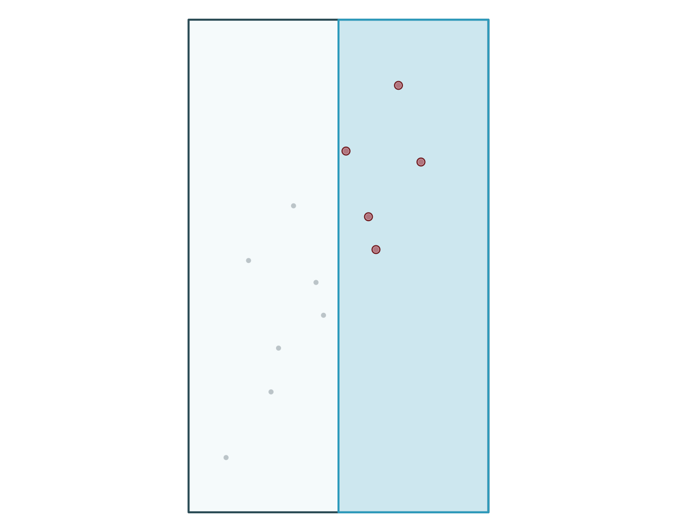
  obs_id track_id seq           timestamp category value
1  OBS03        A   3 2026-03-01 10:00:00   forest    21
2  OBS04        A   4 2026-03-01 11:00:00   forest    24
3  OBS07        B   3 2026-03-02 10:00:00  wetland    17
4  OBS08        B   4 2026-03-02 11:00:00  wetland    18
5  OBS12        C   4 2026-03-03 11:00:00    urban    19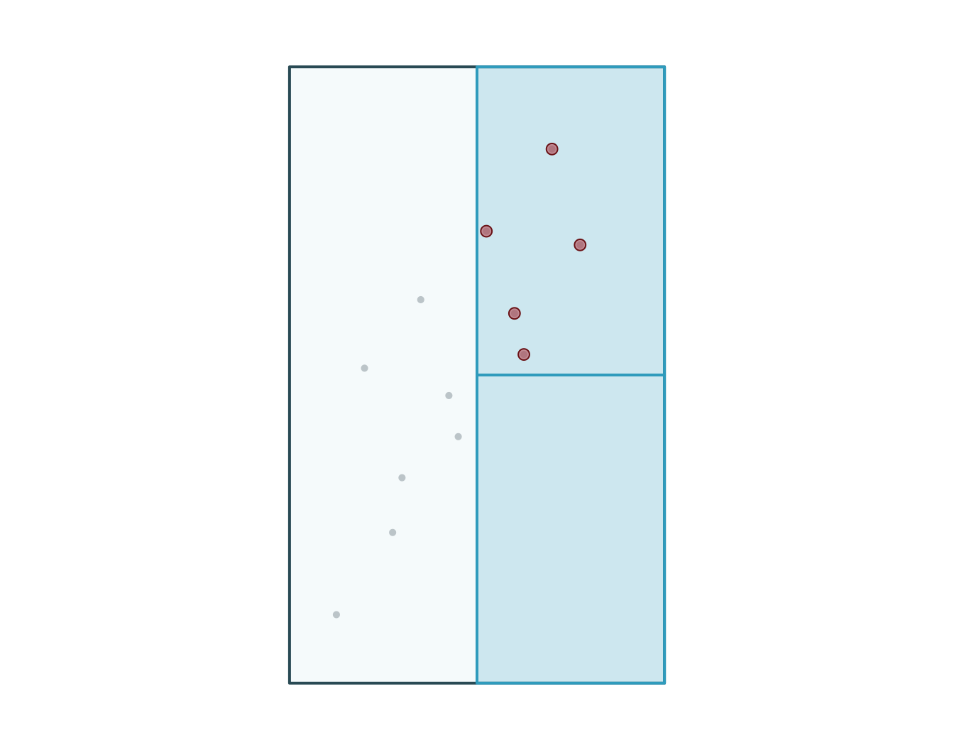
  obs_id track_id seq           timestamp    lon   lat    category value
1  OBS01        A   1 2026-03-01 08:00:00 -72.92 46.78       urban    14
2  OBS02        A   2 2026-03-01 09:00:00 -72.86 46.83       urban    16
3  OBS03        A   3 2026-03-01 10:00:00 -72.79 46.88      forest    21
4  OBS04        A   4 2026-03-01 11:00:00 -72.72 46.94      forest    24
5  OBS05        B   1 2026-03-02 08:00:00 -72.88 46.70 agriculture    11
6  OBS06        B   2 2026-03-02 09:00:00 -72.83 46.76 agriculture    13
  zone_id zone_type
1      NW    forest
2      NW    forest
3      NE     urban
4      NE     urban
5      SW   wetland
6      SW   wetland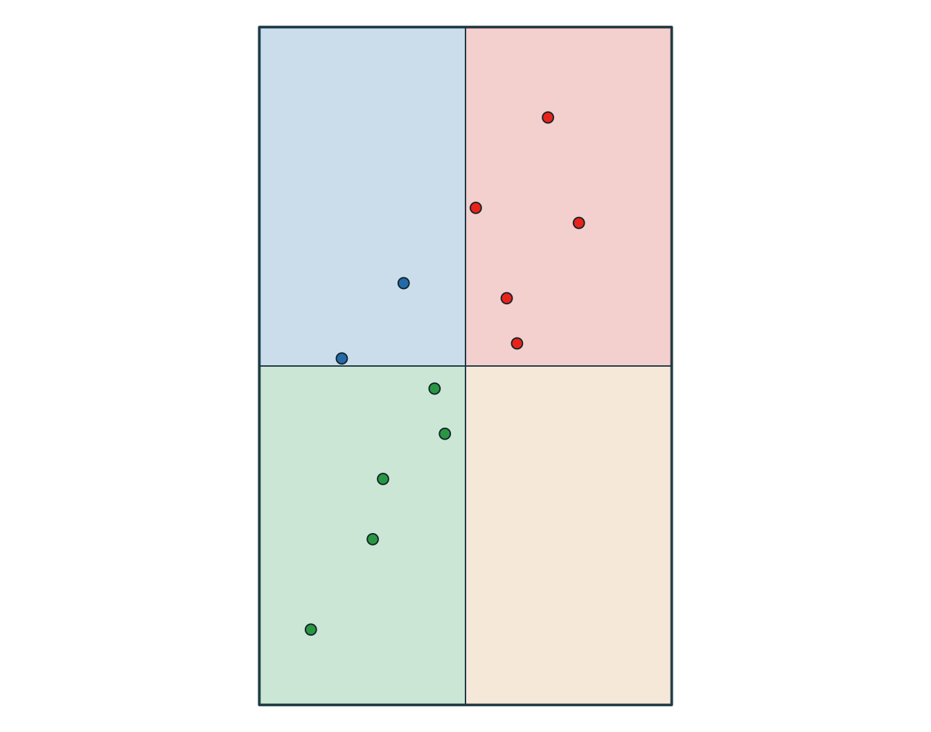
  obs_id track_id seq           timestamp    category value zone_id zone_type
1  OBS01        A   1 2026-03-01 08:00:00       urban    14      NW    forest
2  OBS02        A   2 2026-03-01 09:00:00       urban    16      NW    forest
3  OBS03        A   3 2026-03-01 10:00:00      forest    21      NE     urban
4  OBS04        A   4 2026-03-01 11:00:00      forest    24      NE     urban
5  OBS05        B   1 2026-03-02 08:00:00 agriculture    11      SW   wetland
6  OBS06        B   2 2026-03-02 09:00:00 agriculture    13      SW   wetland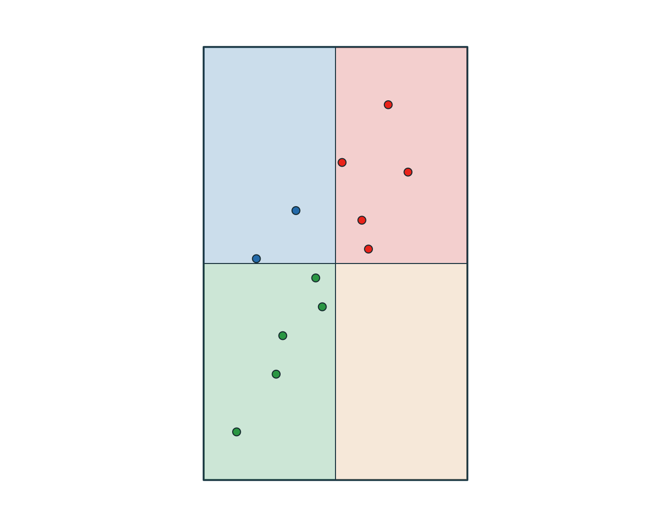
# A tibble: 6 × 3
  track_id zone_id zone_type
  <chr>    <chr>   <chr>
1 A        NW      forest
2 B        NW      forest
3 A        NE      urban
4 B        NE      urban
5 C        NE      urban
6 B SW wetland 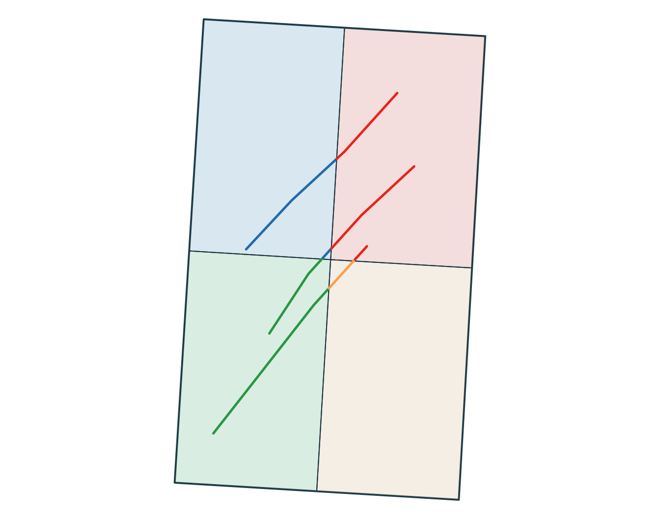
[1] POLYGON
18 Levels: GEOMETRY POINT LINESTRING POLYGON MULTIPOINT ... TRIANGLE
obs_id track_id seq timestamp lon lat category value
1 OBS01 A 1 2026-03-01 08:00:00 -72.92 46.78 urban 14
2 OBS02 A 2 2026-03-01 09:00:00 -72.86 46.83 urban 16
3 OBS03 A 3 2026-03-01 10:00:00 -72.79 46.88 forest 21
4 OBS04 A 4 2026-03-01 11:00:00 -72.72 46.94 forest 24
5 OBS05 B 1 2026-03-02 08:00:00 -72.88 46.70 agriculture 11
6 OBS06 B 2 2026-03-02 09:00:00 -72.83 46.76 agriculture 13
[1] "polygons" obs_id track_id seq timestamp category value
1 OBS01 A 1 2026-03-01 08:00:00 urban 14
2 OBS02 A 2 2026-03-01 09:00:00 urban 16
3 OBS03 A 3 2026-03-01 10:00:00 forest 21
4 OBS04 A 4 2026-03-01 11:00:00 forest 24
5 OBS05 B 1 2026-03-02 08:00:00 agriculture 11
6 OBS06 B 2 2026-03-02 09:00:00 agriculture 13
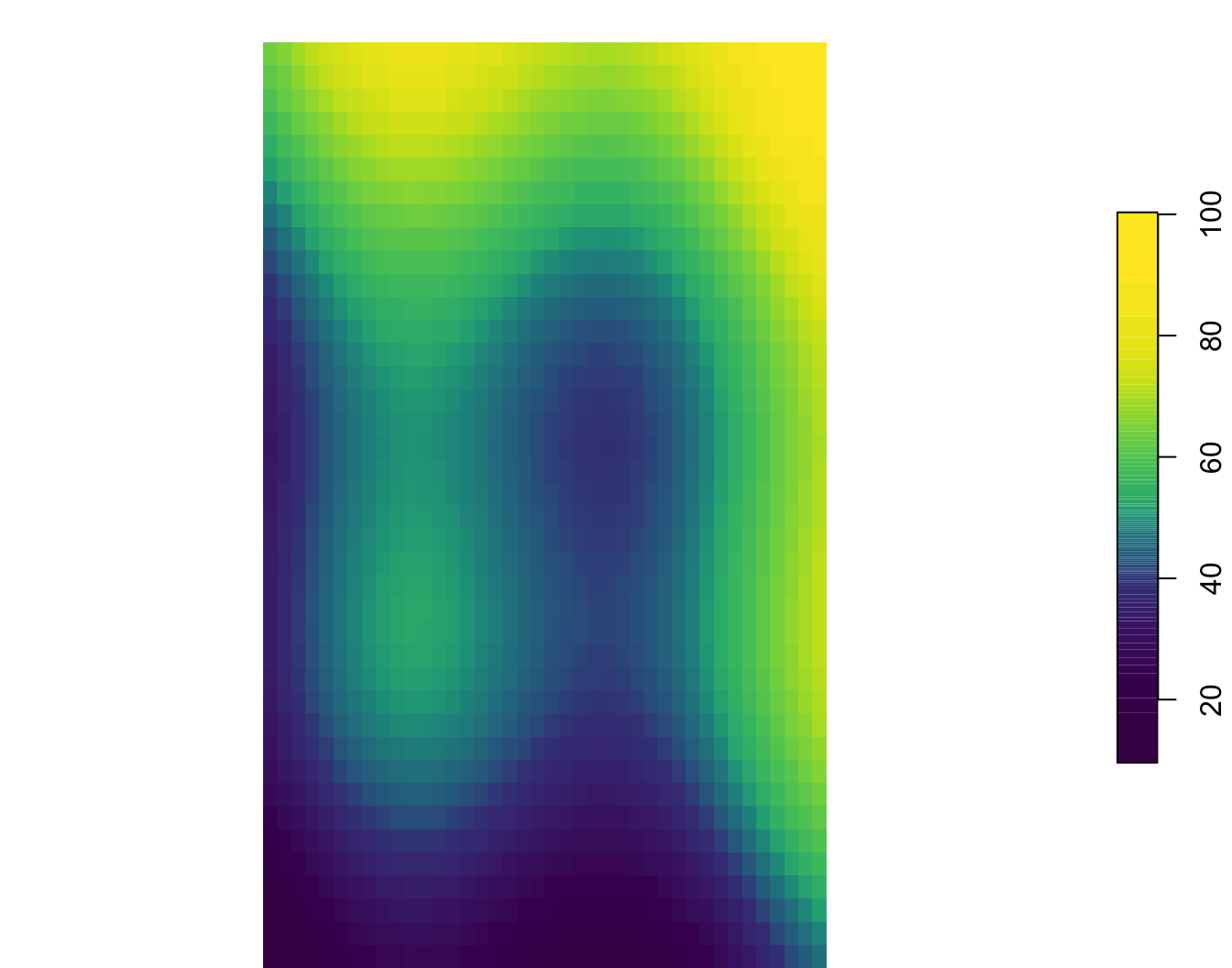
stars object with 2 dimensions and 1 attribute
attribute(s):
Min. 1st Qu. Median Mean 3rd Qu. Max.
surface.tif 9.6 40.8325 48.5 50.00007 59.805 100.32
dimension(s):
from to offset delta refsys point x/y
x 1 40 -73 0.01 WGS 84 FALSE [x]
y 1 40 47 -0.01125 WGS 84 FALSE [y]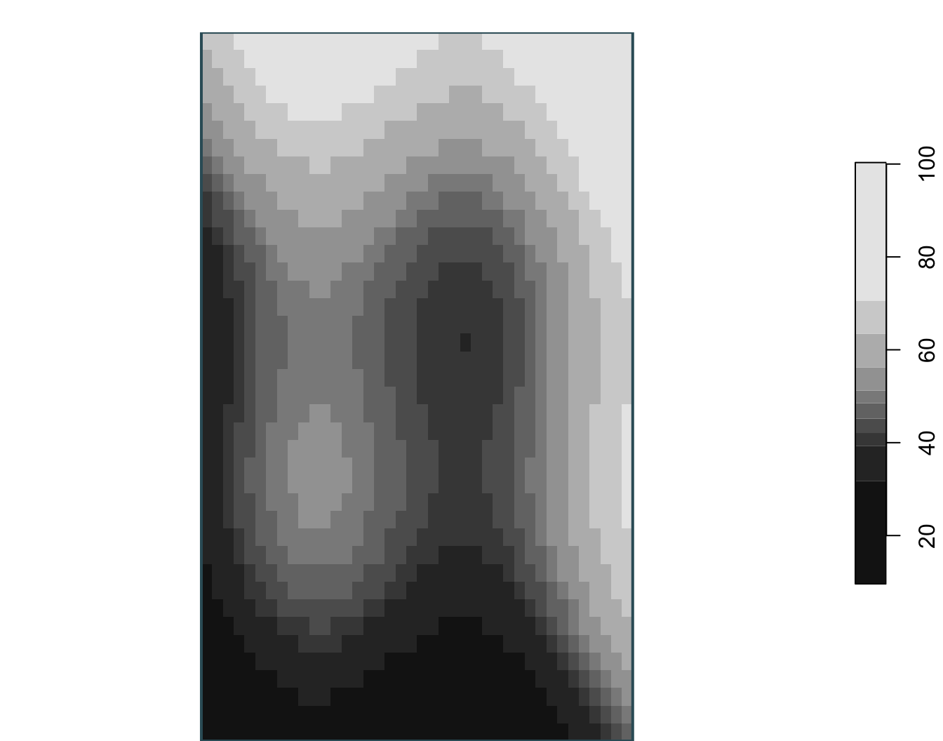
class : SpatRaster
size : 40, 40, 1 (nrow, ncol, nlyr)
resolution : 0.01, 0.01125 (x, y)
extent : -73, -72.6, 46.55, 47 (xmin, xmax, ymin, ymax)
coord. ref. : lon/lat WGS 84 (EPSG:4326)
source : surface.tif
name : surface_value
min value : 9.60
max value : 100.32 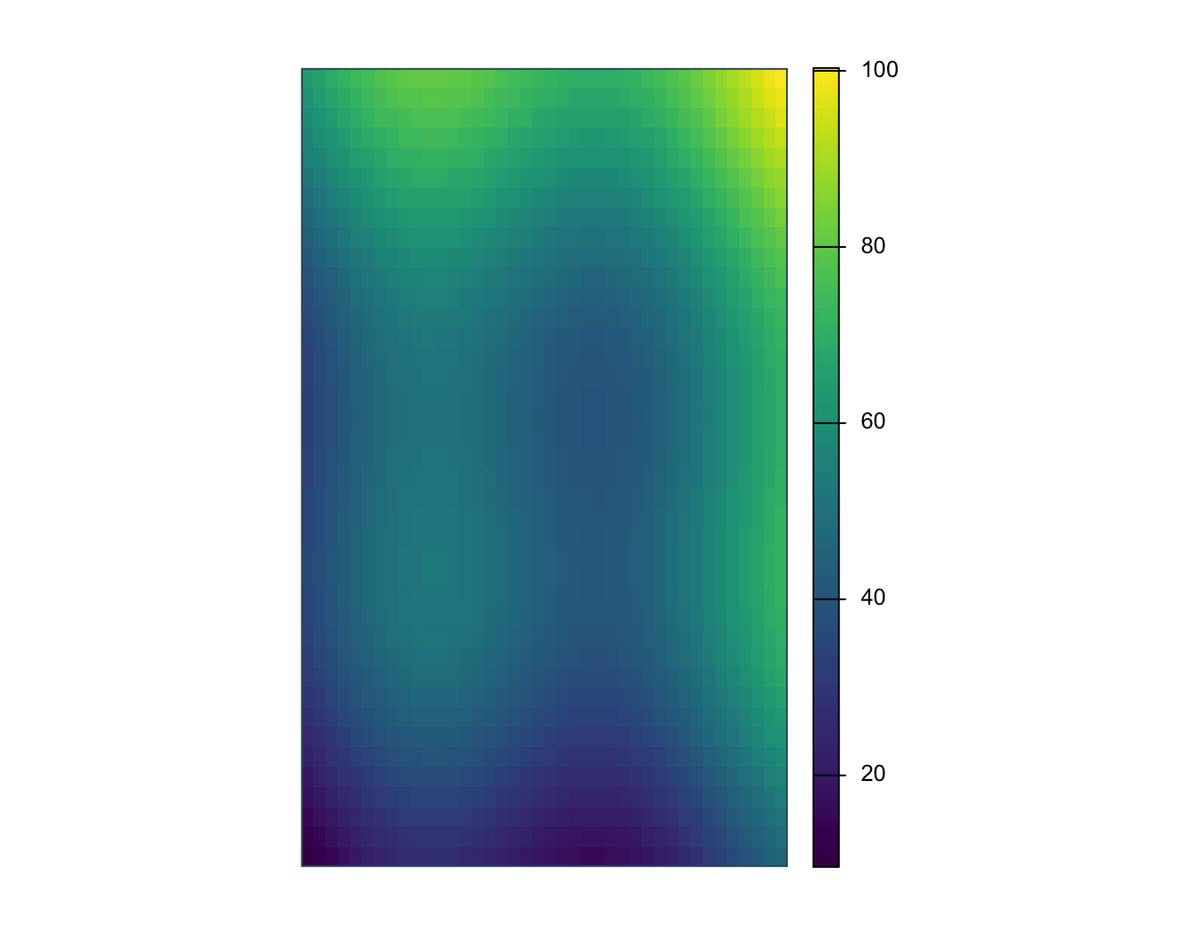
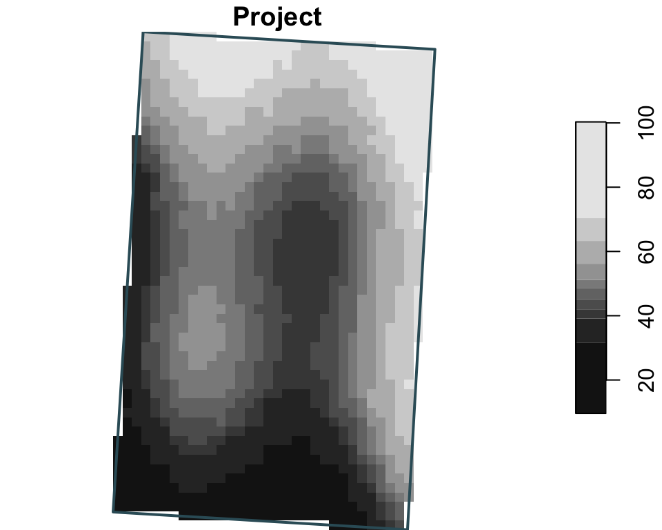
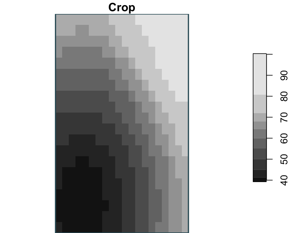
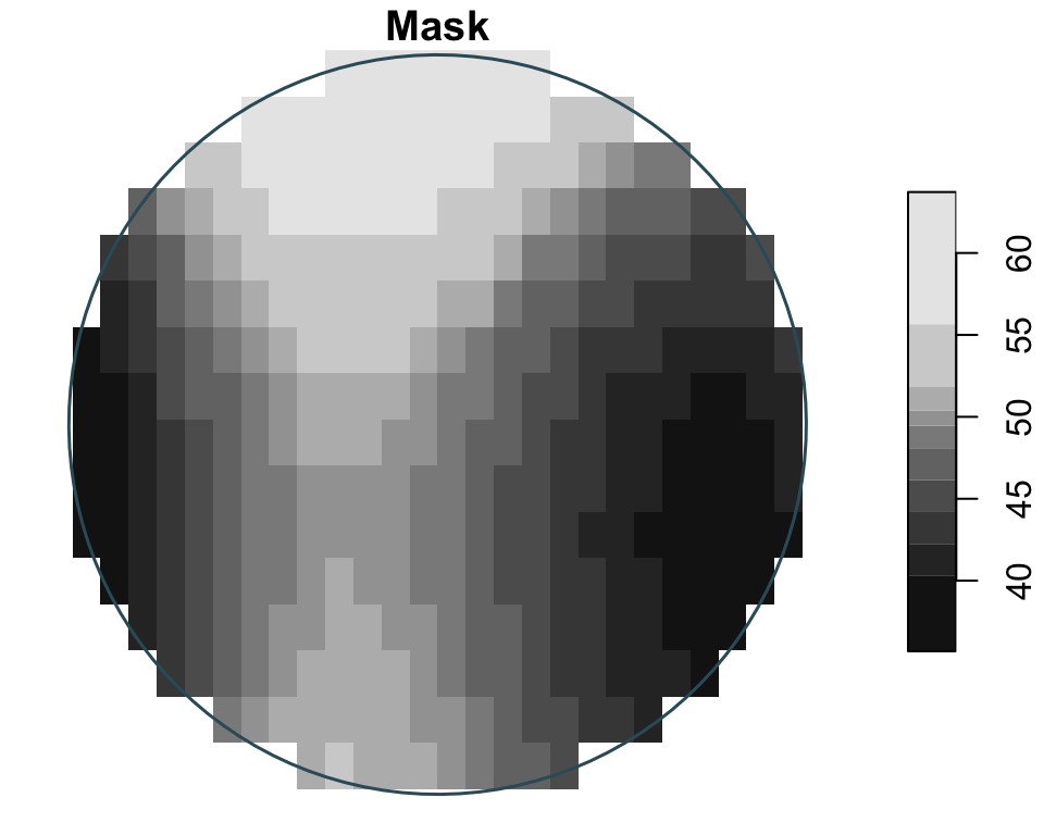
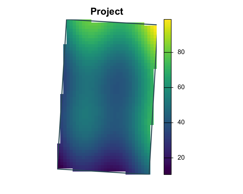
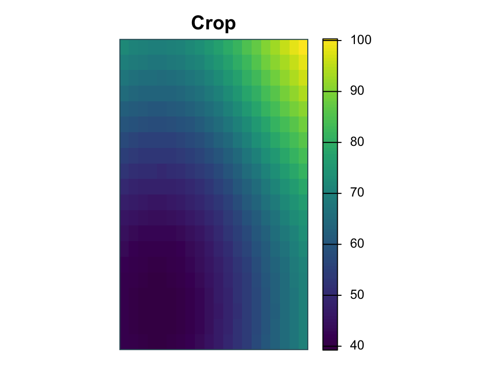
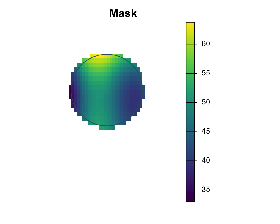
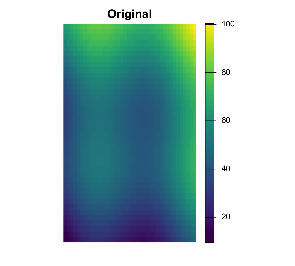
Raster manipulations
Here the three operations are shown independently: project changes CRS, crop uses one zone as the target extent, and mask keeps cells only inside a single buffer geometry.
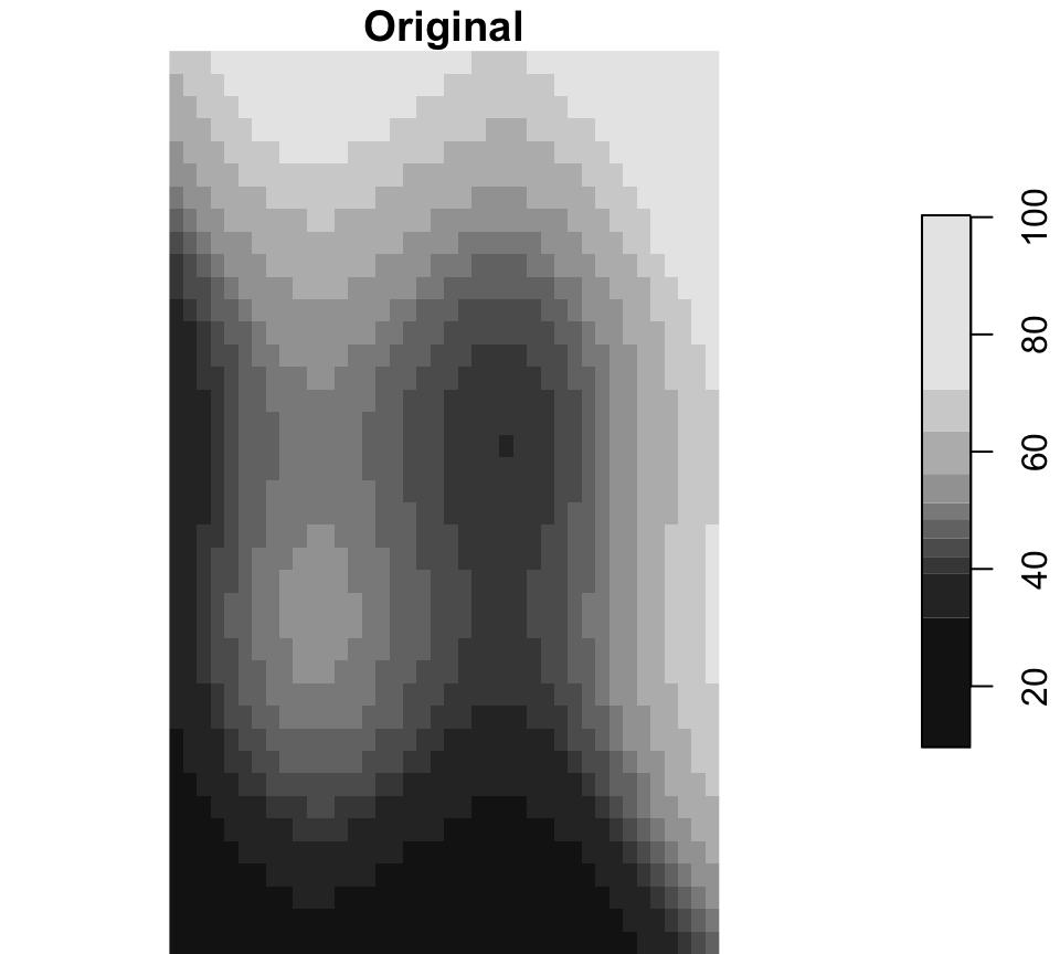
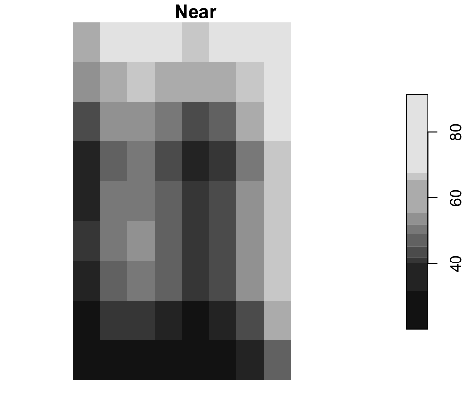
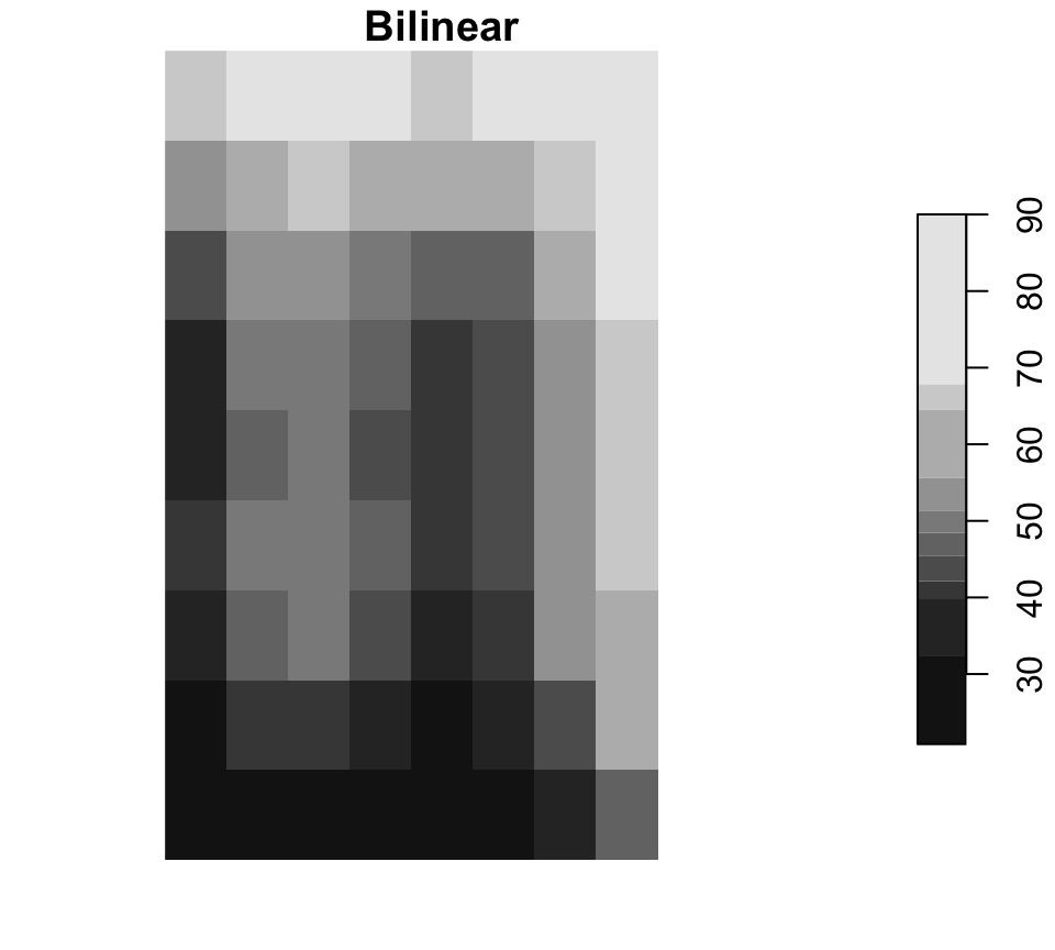
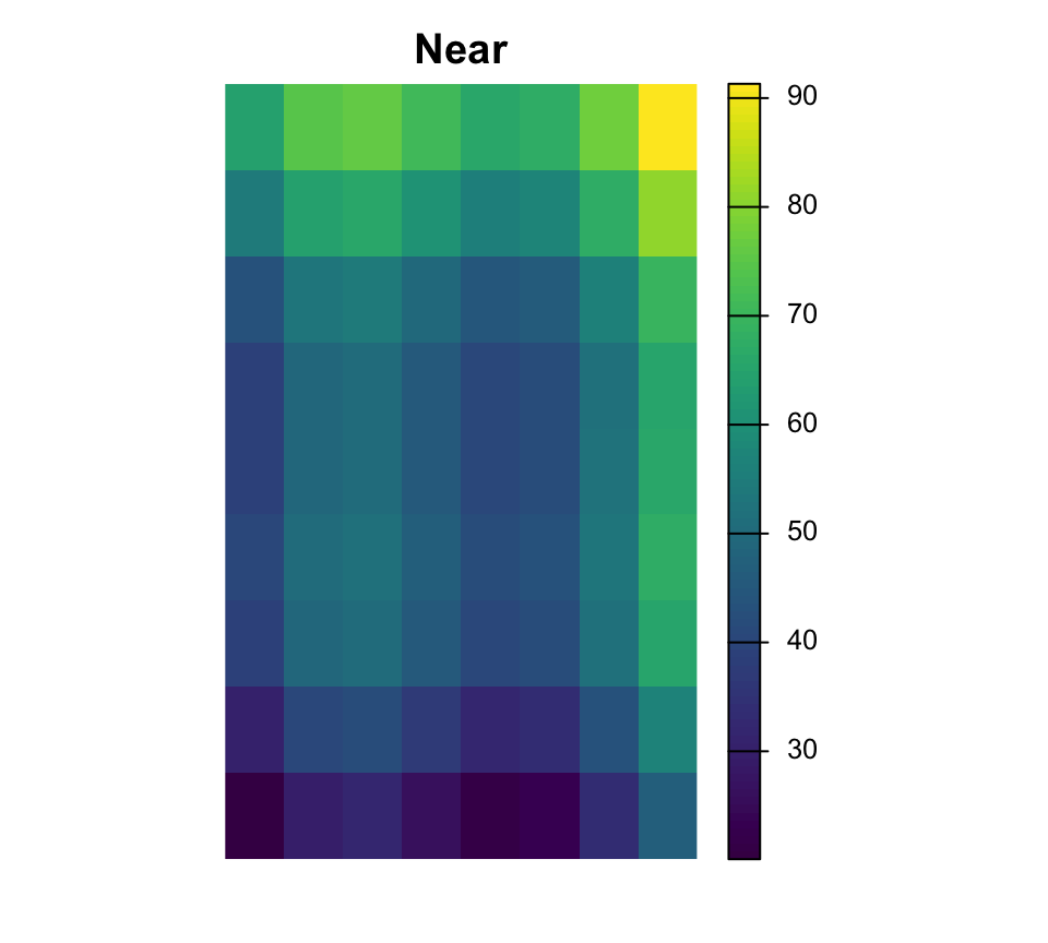
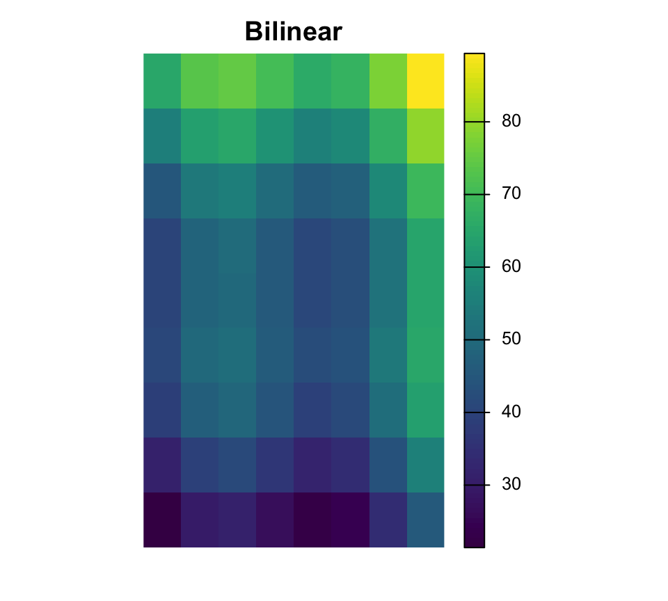
Resampling changes the cell grid
Near is common for categorical rasters, while bilinear is common for continuous surfaces.
[1] "surface.tif" "surface_alt"[1] 2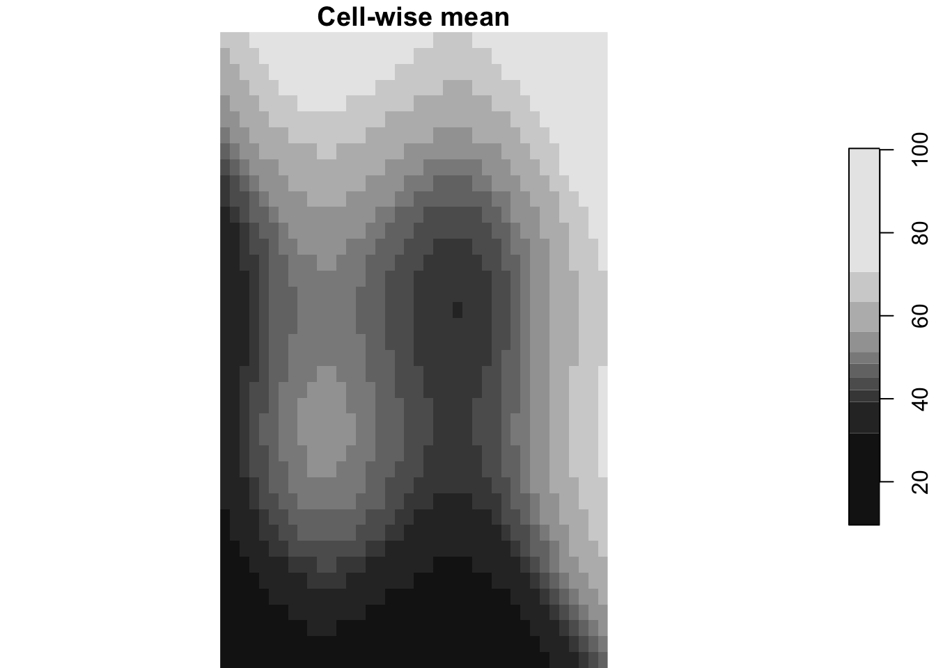
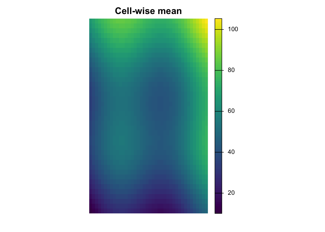
Multi-layer rasters
Can represent bands, variables, or time steps. Cell-wise functions combine information across layers.
  obs_id track_id seq           timestamp    lon   lat    category value
1  OBS01        A   1 2026-03-01 08:00:00 -72.92 46.78       urban    14
2  OBS02        A   2 2026-03-01 09:00:00 -72.86 46.83       urban    16
3  OBS03        A   3 2026-03-01 10:00:00 -72.79 46.88      forest    21
4  OBS04        A   4 2026-03-01 11:00:00 -72.72 46.94      forest    24
5  OBS05        B   1 2026-03-02 08:00:00 -72.88 46.70 agriculture    11
6  OBS06        B   2 2026-03-02 09:00:00 -72.83 46.76 agriculture    13
zone_id zone_type surface_value
1 NW forest 49.71
2 NW forest 48.70
3 NE urban 47.72
4 NE urban 61.39
5 SW wetland 51.67
6 SW wetland 45.88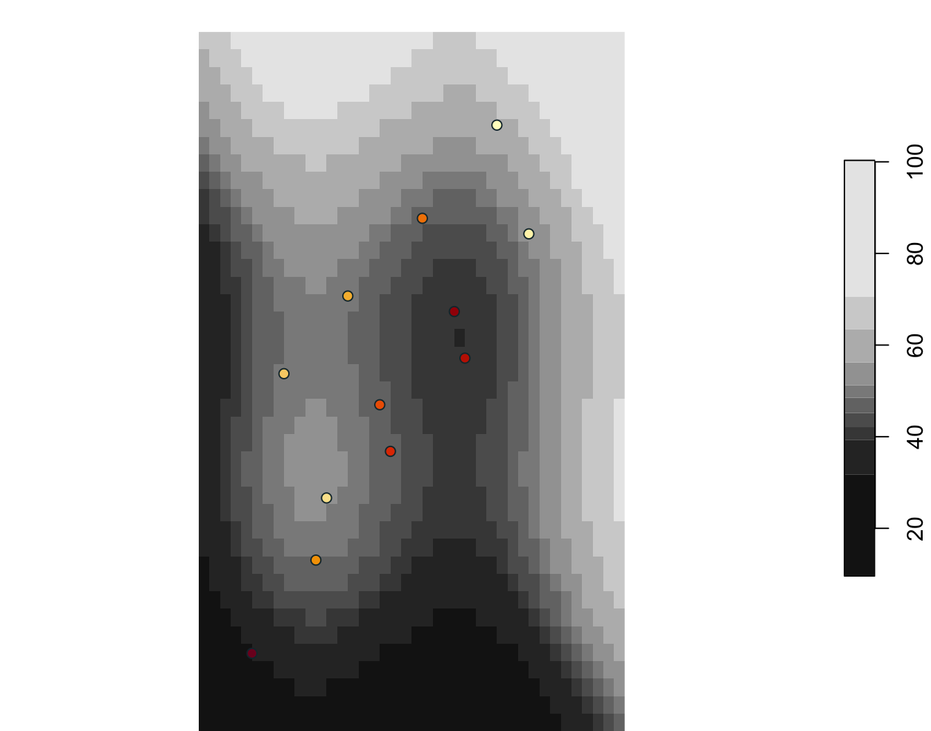
  obs_id zone_id zone_type surface_value
1  OBS01      NW    forest         48.69
2  OBS02      NW    forest         49.60
3  OBS03      NE     urban         47.72
4  OBS04      NE     urban         59.98
5  OBS05      SW   wetland         51.67
6  OBS06      SW   wetland         47.16
# A tibble: 3 × 2
  track_id surface_value
  <chr>            <dbl>
1 A                 50.0
2 B                 45.0
3 C                 44.2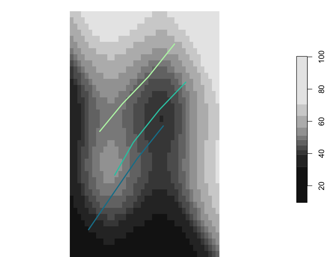
  zone_id   zone_type surface_value
1      NW      forest      55.93852
2      NE       urban      60.33677
3      SW     wetland      39.66305
4      SE agriculture      44.06193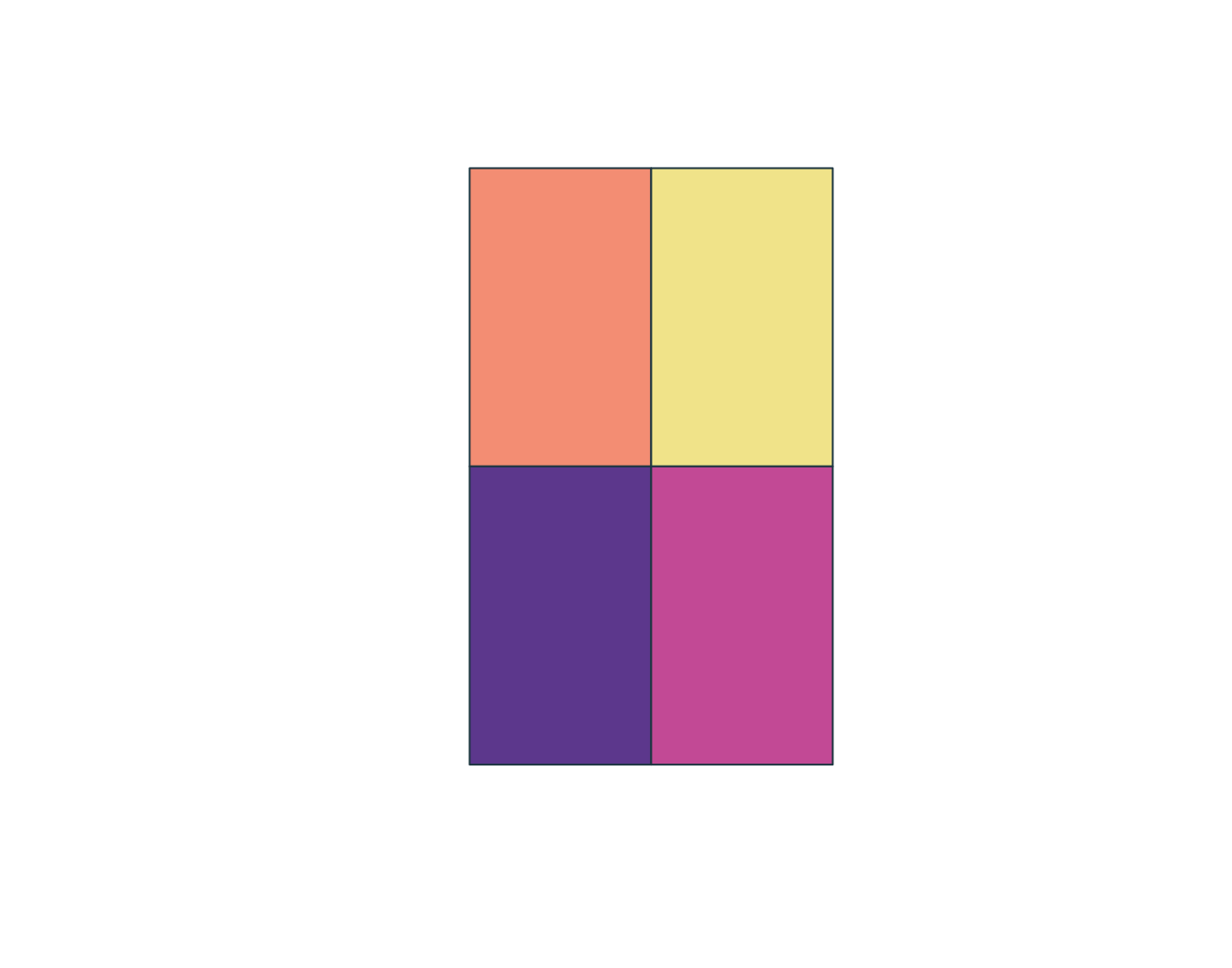
pseudo_points <- st_sample(aoi_qc, size = nrow(points_qc), exact = TRUE) |>
  st_as_sf() |>
  st_join(zones_qc[, c("zone_id", "zone_type")])

pseudo_points$surface_value <- st_extract(surface_qc, pseudo_points)[[1]]
pseudo_points$presence <- 0
points_qc$presence <- 1

pa_data <- bind_rows(points_qc, pseudo_points) |>
  st_drop_geometry() |>
  filter(!is.na(zone_id), !is.na(surface_value))

glm_pa <- glm(presence ~ surface_value + zone_type, family = binomial(), data = pa_data)
term Estimate Std..Error z.value Pr...z..
1 (Intercept) -16.407 3143.229 -0.005 0.996
2 surface_value -0.039 0.036 -1.098 0.272
3 zone_typeforest 19.471 3143.229 0.006 0.995
4 zone_typeurban 18.584 3143.229 0.006 0.995
5 zone_typewetland 18.917 3143.229 0.006 0.995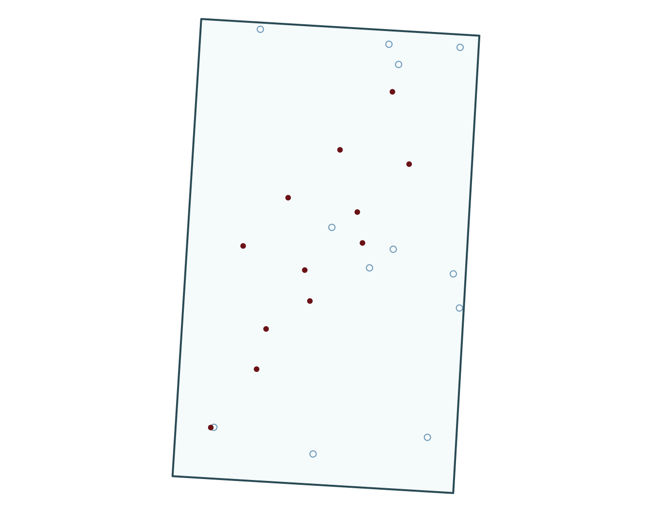
pseudo_points <- spatSample(aoi_qc, size = nrow(points_qc), method = "random", as.points = TRUE)
pseudo_zone <- extract(zones_qc, pseudo_points)
pseudo_surface <- extract(surface_qc, pseudo_points)
pseudo_points <- cbind(pseudo_points, pseudo_zone[, c("zone_id", "zone_type")], pseudo_surface[, "surface_value", drop = FALSE])
pseudo_points$presence <- 0
points_qc$presence <- 1

pa_data <- bind_rows(as.data.frame(points_qc), as.data.frame(pseudo_points)) |>
  filter(!is.na(zone_id), !is.na(surface_value))

glm_pa <- glm(presence ~ surface_value + zone_type, family = binomial(), data = pa_data)
term Estimate Std..Error z.value Pr...z..
1 (Intercept) -13.913 2782.290 -0.005 0.996
2 surface_value -0.061 0.062 -0.981 0.326
3 zone_typeforest 16.642 2782.287 0.006 0.995
4 zone_typeurban 17.569 2782.287 0.006 0.995
5 zone_typewetland 17.009 2782.287 0.006 0.995
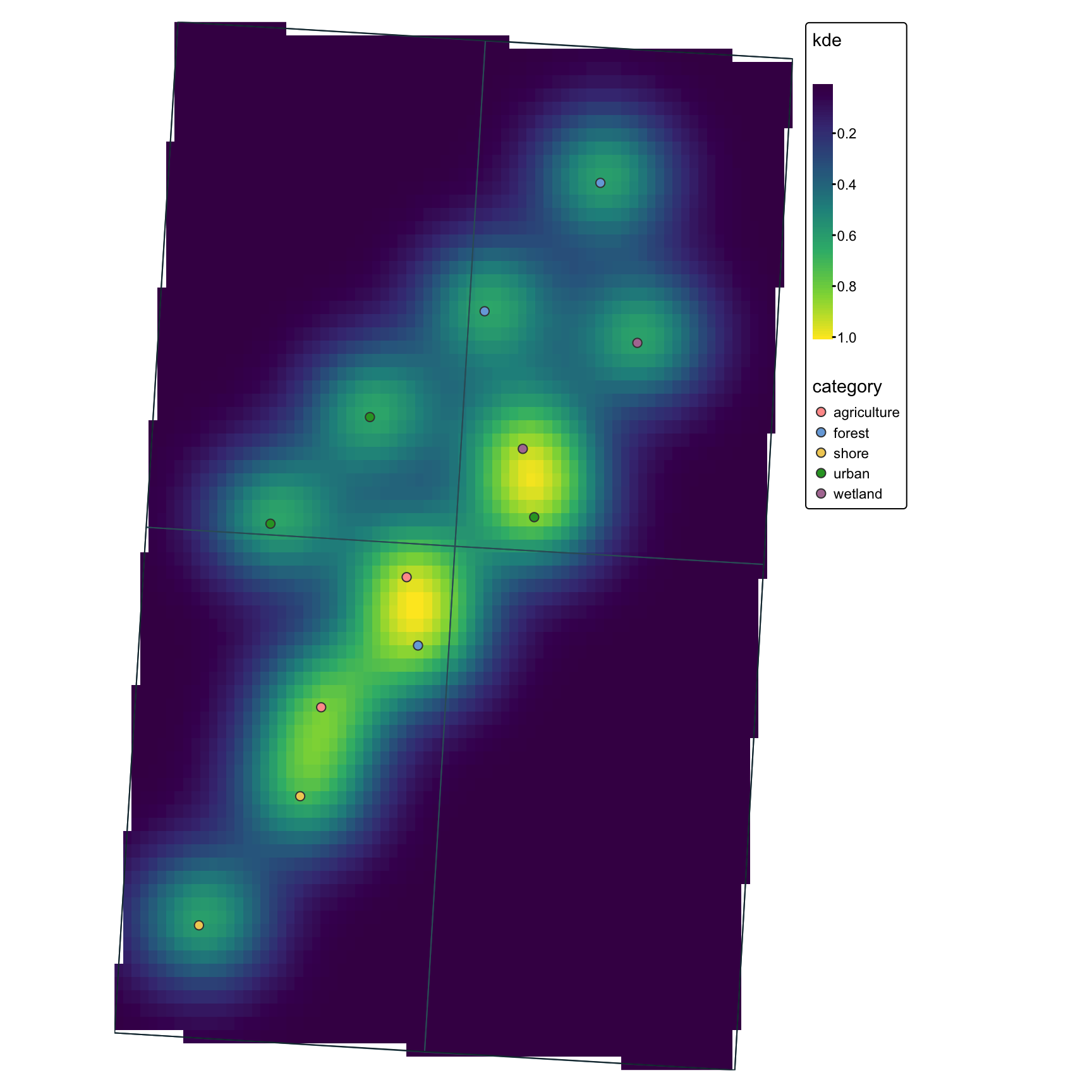
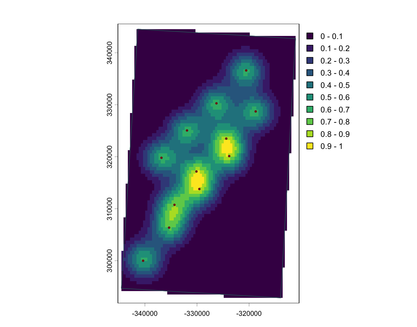
ggplot2ggplot2 works especially well for polished static maps, particularly with sf and stars objects.
gg <- ggplot() +
  geom_stars(
    data = points_kde_sf_plot
  ) +
  scale_fill_viridis_c(name = "KDE") +
  geom_sf(
    data = zones_qc,
    fill = NA,
    color = "#355c67"
  ) +
  geom_sf(
    data = aoi_qc,
    fill = NA,
    color = "#17313b"
  ) +
  geom_sf(
    data = points_sf_qc,
    aes(color = category),
    size = 1.7
   ) +
  coord_sf(expand = FALSE) +
  theme_minimal()
gg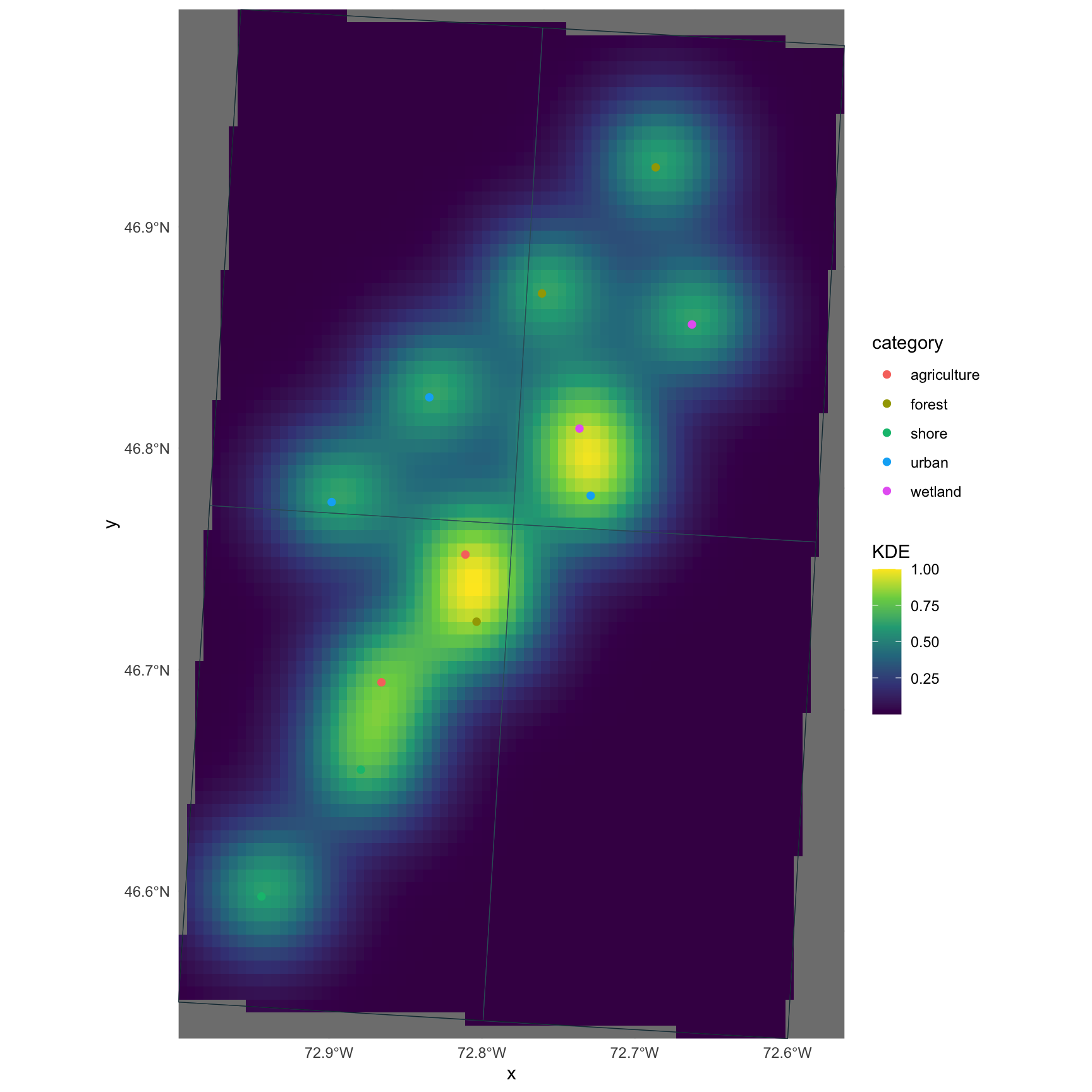
tmaptmap is built for thematic mapping and works well when you want a more map-focused grammar than ggplot2.
tm <- tm_shape(points_kde_sf_plot) +
  tm_raster(col.scale = tm_scale_continuous(
    values = "viridis"
  )) +
  tm_shape(zones_qc) +
  tm_borders(col = "#355c67") +
  tm_shape(points_sf_qc) +
  tm_symbols(
    fill = "category",
    size = 0.5
  ) +
  tm_shape(aoi_qc) +
  tm_borders(col = "#17313b") +
  tm_layout(
    frame = FALSE,
    legend.outside = TRUE
  )
tm